GATE DA

Logistic regression, k-nearest neighbour and naive Bayes

Logistic regression, k-nearest neighbour and naive Bayes are the three basic classifiers in the GATE DA Machine Learning unit. Logistic regression turns a linear score into a probability and is trained by minimising cross-entropy. k-NN predicts from stored data using distances, and naive Bayes from probabilities counted in the training data. Typical questions ask for a class probability from given weights, a gradient or a gradient-descent update, a k-NN vote, or a posterior from a small training table. You need both the formulas and the working habits for each.

4 previous-year questions · 4 solved · 6 practice questions

Logistic regression: the model

Convention used throughout: $x$ is a feature vector, $w$ the weight vector, $b$ the bias. Labels are $y \in {0, 1}$ ; a variant with labels in ${- 1, + 1}$ is noted where it changes a formula. Samples are the rows of $X$ , $p_{i}$ is the model's predicted probability of class 1 for sample $i$ , $σ (\cdot)$ always means the sigmoid, and $ln$ is the natural logarithm. Despite its name, logistic regression is a classifier. It models the probability of class 1 by passing a linear score $z = w^{⊤} x + b$ through the sigmoid.

SIGMOID (LOGISTIC FUNCTION)

σ (z) = \frac{1}{1 + e ^{- z}}

The output lies in (0, 1). $σ (0) = 0.5$ ; $σ (z) \to 1$ as $z \to \infty$ and $σ (z) \to 0$ as $z \to - \infty$ .

SIGMOID IDENTITIES

σ (- z) = 1 - σ (z), σ^{'} (z) = σ (z) (1 - σ (z))

The derivative is at most 0.25, reached at $z = 0$ . This identity is what makes the gradient of the cross-entropy loss so simple.

LOGISTIC REGRESSION MODEL

P (y = 1 ∣ x) = σ (w^{⊤} x + b), P (y = 0 ∣ x) = 1 - P (y = 1 ∣ x)

Binary classification. The prediction is class 1 when this probability exceeds the chosen threshold, which is 0.5 unless the question states another.

LOG-ODDS (LOGIT) IS LINEAR

ln \frac{P ( y = 1 ∣ x )}{1 - P ( y = 1 ∣ x )} = w^{⊤} x + b

With the other features fixed, each unit increase in $x_{j}$ adds $w_{j}$ to the log-odds, which multiplies the odds by $e^{w_{j}}$ .

DECISION BOUNDARY

w^{⊤} x + b = ln \frac{t}{1 - t} (threshold t), w^{⊤} x + b = 0 for t = 0.5

The boundary is a hyperplane, so logistic regression is a linear classifier. $w$ is normal to the boundary and points towards the class-1 side. Changing $t$ moves the hyperplane parallel to itself.

EXAM TIP

To classify at threshold 0.5 you do not need the sigmoid: check the sign of $w^{⊤} x + b$ . Compute $σ$ only when the question asks for the probability itself.

Logistic regression: loss, gradient and training

The weights are found by maximum likelihood, which is the same as minimising the cross-entropy (log-loss). There is no closed-form solution, so gradient descent or a similar iterative method is used. The loss is convex in $(w, b)$ , so gradient descent cannot get stuck in a bad local minimum. If the training data are linearly separable, however, no finite minimiser exists (see the list below).

LOG-LIKELIHOOD

ℓ (w, b) = i = 1 \sum n [y_{i} ln p_{i} + (1 - y_{i}) ln (1 - p_{i})], J (w, b) = - \frac{1}{n} ℓ (w, b)

Each sample contributes $ln P (y_{i} ∣ x_{i})$ . Maximising $ℓ$ and minimising $J$ give the same weights.

CROSS-ENTROPY LOSS (NATURAL LOG)

J (w, b) = - \frac{1}{n} i = 1 \sum n [y_{i} ln p_{i} + (1 - y_{i}) ln (1 - p_{i})], p_{i} = σ (w^{⊤} x_{i} + b)

For one sample the loss is $- ln p$ if $y = 1$ and $- ln (1 - p)$ if $y = 0$ . Using $lo g_{2}$ instead only multiplies the loss by a constant.

THE SAME LOSS WITH LABELS IN {−1, +1}

J (w, b) = \frac{1}{n} i = 1 \sum n ln (1 + e^{- y_{i} z_{i}}), z_{i} = w^{⊤} x_{i} + b, y_{i} \in {- 1, + 1}

This is identical to the cross-entropy above, rewritten for $\pm 1$ labels using $σ (- z) = 1 - σ (z)$ . Check which label convention a question uses before you substitute.

GRADIENT OF THE LOSS

\frac{\partial J}{\partial w} = \frac{1}{n} i = 1 \sum n (p_{i} - y_{i}) x_{i} = \frac{1}{n} X^{⊤} (p - y), \frac{\partial J}{\partial b} = \frac{1}{n} i = 1 \sum n (p_{i} - y_{i})

Labels in ${0, 1}$ . This has the same form as linear regression's gradient when that loss is written $\frac{1}{2 n} \sum (\overset{y}{^}_{i} - y_{i})^{2}$ , with $p_{i}$ in place of the linear prediction. For a single sample, drop the $\frac{1}{n}$ and the sum.

L2-REGULARISED LOSS AND GRADIENT

J_{λ} (w, b) = J (w, b) + \frac{λ}{2 n} ∥ w ∥^{2}, \frac{\partial J _{λ}}{\partial w} = \frac{1}{n} X^{⊤} (p - y) + \frac{λ}{n} w

$λ \geq 0$ sets the strength of the penalty. The bias is usually not penalised, so $\partial J_{λ} / \partial b$ is unchanged. Books scale $λ$ differently (with or without $\frac{1}{n}$ or $\frac{1}{2}$ ), so use the form the question gives.

GRADIENT DESCENT UPDATE

w \leftarrow w - η \frac{\partial J}{\partial w}, b \leftarrow b - η \frac{\partial J}{\partial b}

$η > 0$ is the learning rate. With the squared-error loss $\frac{1}{2} (p - y)^{2}$ per sample instead, the gradient picks up an extra factor $p (1 - p)$ . Learning then slows when the sigmoid saturates, and the loss is no longer convex in $w$ .

Facts worth remembering

The sign of $p_{i} - y_{i}$ gives the direction of the update. If $y = 1$ and $p$ is small, the update $w \leftarrow w + η (1 - p) x_{i}$ moves the weights along $+ x_{i}$ .
If the training data are linearly separable, the likelihood keeps rising as $∥ w ∥ \to \infty$ , so the unregularised weights never converge. An L2 penalty fixes this.
Changing the threshold moves the decision boundary parallel to itself, so the model is a linear classifier at every threshold.
For more than two classes, the softmax replaces the sigmoid: $P (y = k ∣ x) = e^{z_{k}} / \sum_{j} e^{z_{j}}$ with $z_{k} = w_{k}^{⊤} x + b_{k}$ .

WORKED EXAMPLE

A logistic regression model has $w = (2, - 1)$ and $b = - 1$ . For the sample $x = (1, 2)$ with label $y = 1$ : (a) find $P (y = 1 ∣ x)$ ; (b) do one gradient-descent step on this single sample with $η = 0.5$ , and give the new weights and bias.

Solution

$z = 2 (1) + (- 1) (2) - 1 = - 1$ , so $p = σ (- 1) = \frac{1}{1 + e} \approx 0.2689$ . The model predicts class 0, but the label is 1.
$p - y = 0.2689 - 1 = - 0.7311$ .
$\partial J / \partial w = (p - y) x = - 0.7311 (1, 2) = (- 0.7311, - 1.4621)$ and $\partial J / \partial b = - 0.7311$ .
$w \leftarrow (2, - 1) - 0.5 (- 0.7311, - 1.4621) = (2.3655, - 0.2689)$ .
$b \leftarrow - 1 - 0.5 (- 0.7311) = - 0.6345$ (to 4 d.p.).
Check: the new score is $z = 2.3655 - 2 (0.2689) - 0.6345 \approx 1.193$ , so $σ (1.193) \approx 0.767$ .

Answer: (a) $p \approx 0.269$ . (b) $w \approx (2.366, - 0.269)$ and $b \approx - 0.634$ . The probability for this sample rises to about 0.767.

k-nearest neighbour: the method

k-NN is a lazy, non-parametric method: training only stores the data. To predict for a query point, find the $k$ training points closest to it. For classification, take the majority class among them; for regression, take their average. Use Euclidean distance unless the question says otherwise.

EUCLIDEAN, MANHATTAN, MINKOWSKI AND CHEBYSHEV DISTANCE

d_{2} (a, b) = j \sum (a_{j} - b_{j})^{2}, d_{1} (a, b) = j \sum ∣ a_{j} - b_{j} ∣, d_{r} (a, b) = (j \sum ∣ a_{j} - b_{j} ∣^{r})^{1/ r}, d_{\infty} (a, b) = j max ∣ a_{j} - b_{j} ∣

Euclidean is $r = 2$ , Manhattan is $r = 1$ , and Chebyshev is the limit $r \to \infty$ . $d_{r}$ is a metric for $r \geq 1$ . The order is written $r$ here because $p$ means a predicted probability in these notes. The nearest neighbour can change from one metric to another, so always use the one the question names.

K-NN REGRESSION

\overset{y}{^} (x) = \frac{1}{k} i \in N_{k} (x) \sum y_{i}

$N_{k} (x)$ is the set of the $k$ nearest training points. A distance-weighted version uses weights proportional to $1/ d$ . A query that coincides with a training point ( $d = 0$ ) is usually given that point's value.

Procedure for a k-NN classification question

Scale the features first if the question says so.
Compute the distance from the query to every training point. Squared distances give the same ordering and save the square root.
Sort the distances and pick the $k$ smallest. If two points tie for the $k$ -th place, follow the question's rule.
Count the class labels among the $k$ neighbours. The majority class is the prediction.
If the vote ties, follow the question's rule (a smaller $k$ , the nearest neighbour's class, or a fixed class). In a two-class problem an odd $k$ prevents vote ties. It does not prevent ties in distance.

Choice of k	Effect
$k = 1$	Training error is zero, because each training point is its own nearest neighbour at distance 0. This holds unless identical feature vectors carry different labels. The boundary is jagged: high variance, sensitive to noise.
Small $k$	Low bias, high variance: overfitting.
Large $k$	High bias, low variance: a smoother boundary, with a risk of underfitting.
$k = n$	Every query gets the overall majority class (the global mean in regression), with unweighted votes.

k-NN works from distances, so a feature with a large numeric range dominates the others. Feature scaling (min–max or standardisation) puts the features on a comparable footing. Irrelevant features and high dimension also hurt: in many dimensions, the distances from a query to all points become similar and so less informative. This is the curse of dimensionality. Prediction is slow: a brute-force search touches all $n$ stored points, costing $O (n d)$ per query for $d$ features.

MIN-MAX AND Z-SCORE SCALING

x^{'} = \frac{x - x _{m i n}}{x _{m a x} - x _{m i n}}, x^{'} = \frac{x - x ˉ}{s}

$\overset{x}{ˉ}$ and $s$ are the mean and standard deviation of the feature. Compute $x_{m i n}$ , $x_{m a x}$ , $\overset{x}{ˉ}$ and $s$ from the training data, and apply the same values to the query.

Further facts

The 1-NN decision boundary is made of pieces of the perpendicular bisectors between training points of different classes: the faces of the Voronoi cells around the training points.
As $n \to \infty$ (with i.i.d. data and smooth class densities), the error rate of 1-NN is at most twice the Bayes error rate, the lowest error any classifier can achieve.
For categorical features, Hamming distance (the number of features that differ) is the usual choice.

EXAM TIP

In leave-one-out evaluation, the point being tested is removed from its own neighbour set. Forgetting this gives it a distance of 0 to itself and a wrong vote.

Naive Bayes classifier

Naive Bayes applies Bayes' theorem with one strong assumption: given the class, the features are conditionally independent. That turns a hard joint likelihood into a product of one-feature terms, each easy to estimate by counting.

NAIVE BAYES POSTERIOR

P (c ∣ x_{1}, \dots, x_{d}) = \frac{P ( c ) \prod _{j = 1}^{d} P ( x _{j} ∣ c )}{\sum _{c^{'}} P ( c ^{'} ) \prod _{j = 1}^{d} P ( x _{j} ∣ c ^{'} )}

This assumes the features are conditionally independent given the class. The denominator is the same for every class, so you need it only when the question asks for an actual probability.

NAIVE BAYES DECISION RULE (MAP)

\overset{c}{^} = ar g c max P (c) j = 1 \prod d P (x_{j} ∣ c)

Compare the unnormalised scores. In practice the logs are summed, $ln P (c) + \sum_{j} ln P (x_{j} ∣ c)$ , to avoid numerical underflow. With equal priors, the rule reduces to picking the class with the largest likelihood (maximum likelihood).

ESTIMATES FROM COUNTS

P (c) = \frac{N _{c}}{N}, P (x_{j} = v ∣ c) = \frac{N _{j, v, c}}{N _{c}}

$N_{c}$ is the number of training samples in class $c$ , and $N_{j, v, c}$ is how many of them have feature $j$ equal to $v$ . These are maximum-likelihood estimates and can be zero. Priors are smoothed only if the question says so.

LAPLACE (ADD-$\ALPHA$) SMOOTHING

P (x_{j} = v ∣ c) = \frac{N _{j, v, c} + α}{N _{c} + α V _{j}}

$V_{j}$ is the number of distinct values feature $j$ can take (2 for a binary feature). $α = 1$ is Laplace smoothing. It stops a single unseen value from forcing the whole product to zero.

MULTINOMIAL NAIVE BAYES (WORD COUNTS)

P (w ∣ c) = \frac{count ( w , c ) + α}{\sum _{w^{'}} count ( w ^{'} , c ) + α ∣ V ∣}, score (c) = P (c) w \prod P (w ∣ c)^{n_{w}}

Used for text classification. $count (w, c)$ is the number of times word $w$ appears across the training documents of class $c$ , $∣ V ∣$ is the vocabulary size, and $n_{w}$ is how often $w$ occurs in the document being classified.

GAUSSIAN NAIVE BAYES

p (x_{j} ∣ c) = \frac{1}{2 π σ _{j c}^{2}} exp (- \frac{( x _{j} - μ _{j c} ) ^{2}}{2 σ _{j c}^{2}})

For continuous features. $μ_{j c}$ and $σ_{j c}^{2}$ are the mean and variance of feature $j$ within class $c$ (here $σ_{j c}$ is a standard deviation, not the sigmoid). The maximum-likelihood variance divides by $N_{c}$ and the unbiased one by $N_{c} - 1$ ; use the one the question states. The result is a density, so it can exceed 1. Multiply the terms together as before.

NUMBER OF PARAMETERS (D BINARY FEATURES, K CLASSES)

naive Bayes: (K - 1) + K d, full joint model: (K - 1) + K (2^{d} - 1)

The independence assumption makes the parameter count grow linearly in $d$ instead of exponentially. The $K - 1$ term counts the priors, since they sum to 1.

Procedure for a training-table question

Count the samples in each class to get the priors $P (c)$ .
For each class and each feature value in the query, count the matching rows to get $P (x_{j} ∣ c)$ . Add smoothing if the question asks for it.
Multiply the prior by the likelihoods to get one score per class.
Pick the class with the largest score. For a posterior, divide that class's score by the sum of all the scores.

WORKED EXAMPLE

A training set of six emails has two binary features: Free (the word 'free' is present) and Win (the word 'win' is present). Rows (Free, Win, class): (Y,Y,Spam), (Y,N,Spam), (Y,Y,Spam), (N,N,Ham), (Y,N,Ham), (N,Y,Ham). Classify a new email with Free = Y and Win = Y, and give the posterior probability of Spam (a) without smoothing and (b) with Laplace smoothing $α = 1$ on the likelihoods.

Solution

Priors: $P (Spam) = 3/6$ and $P (Ham) = 3/6$ .
(a) Spam: $P (Free = Y ∣ Spam) = 3/3$ and $P (Win = Y ∣ Spam) = 2/3$ , so the score is $\frac{1}{2} \cdot 1 \cdot \frac{2}{3} = \frac{1}{3}$ .
Ham: $P (Free = Y ∣ Ham) = 1/3$ and $P (Win = Y ∣ Ham) = 1/3$ , so the score is $\frac{1}{2} \cdot \frac{1}{9} = \frac{1}{18}$ .
Posterior of Spam $= \frac{1/3}{1/3 + 1/18} = \frac{6}{7} \approx 0.857$ .
(b) The features are binary, so add 1 to each numerator and 2 to each denominator. Spam: $\frac{4}{5} \cdot \frac{3}{5} \cdot \frac{1}{2} = \frac{6}{25}$ . Ham: $\frac{2}{5} \cdot \frac{2}{5} \cdot \frac{1}{2} = \frac{2}{25}$ .
Posterior of Spam $= \frac{6/25}{6/25 + 2/25} = 0.75$ .

Answer: (a) $6/7 \approx 0.857$ ; (b) $0.75$ . Both classify the email as Spam. Here, smoothing pulls the posterior towards 0.5.

EXAM TIP

Naive Bayes can rank the classes correctly even when the independence assumption is false. Its posterior probabilities can then be unreliable, typically pushed towards 0 or 1 when correlated features count the same evidence twice. Priors matter too: a rare class needs a strong likelihood to win.

Comparing the three and common traps

Property	Logistic regression	k-NN	Naive Bayes
Type	Discriminative (models $P (y ∣ x)$ ), parametric	Instance-based, non-parametric	Generative (models $P (x ∣ c) P (c)$ ), parametric
What is learned	$w$ and $b$ , by gradient descent	Nothing (stores the data)	Priors and per-feature likelihoods, by counting
Decision boundary	Linear	Flexible, locally defined (piecewise linear for 1-NN)	Linear for binary or one-hot categorical features, and for Gaussian features with variances shared across classes. Quadratic for Gaussian features with class-specific variances.
Main hyperparameters	Learning rate, regularisation strength	$k$ , distance metric	Smoothing $α$
Needs feature scaling	Helps gradient descent converge; matters when weights are regularised	Essential	No (Gaussian naive Bayes uses per-class variances)
Prediction cost per query	$O (d)$	$O (n d)$ by brute force: touches every stored point	$O (K d)$
Key assumption	Log-odds are linear in the features	Nearby points share a label	Features are independent given the class

Traps to avoid

Logistic regression predicts a class probability. It is not a regression model for a continuous target.
A sigmoid output of 0.5 corresponds to log-odds 0, that is $w^{⊤} x + b = 0$ , not $w^{⊤} x + b = 0.5$ .
In the gradient the error term is $p - y$ (prediction minus label). Flipping the sign makes the update move the wrong way.
Check whether the labels are ${0, 1}$ or ${- 1, + 1}$ before you use a loss or gradient formula.
k-NN with $k = 1$ has zero training error, but that says nothing about test error.
Squared distances are fine for ranking neighbours, but not as the $d$ in a $1/ d$ -weighted vote.
In naive Bayes a zero count gives a zero likelihood that wipes out the whole product unless smoothing is used. The amount added to the denominator is $α V_{j}$ , not $α$ .
Do not drop the prior $P (c)$ when the classes in the training table are imbalanced.

PREVIOUS-YEAR QUESTIONS

4 questions from the DA papers

Try each question first, then open the answer. We placed each question under a topic ourselves; the exam paper does not label topics.

See these papers in full: GATE DA 2025 · GATE DA 2024

GATE 2025 DA Q.35

GATE 2025 · DAQ.35 · 1 mark · NAT

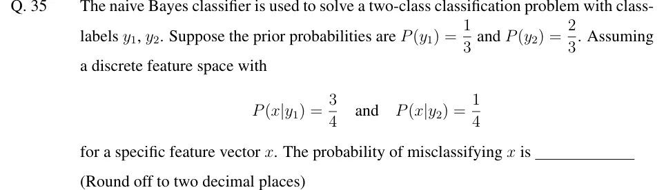
The naive Bayes classifier is used to solve a two-class classification problem with class-labels $y_{1}$ , $y_{2}$ . Suppose the prior probabilities are $P (y_{1}) = \frac{1}{3}$ and $P (y_{2}) = \frac{2}{3}$ . Assuming a discrete feature space with

P (x ∣ y_{1}) = \frac{3}{4} and P (x ∣ y_{2}) = \frac{1}{4}

for a specific feature vector $x$ . The probability of misclassifying $x$ is ______ (Round off to two decimal places)

Answer and solution

GATE 2025 DA Q.35: answer and solution

See the question in the paper

Tap to open full size

GATE 2025 DA Q.35: answer and solution

GATE 2024 DA Q.18

GATE 2024 · DAQ.18 · 1 mark · MCQ

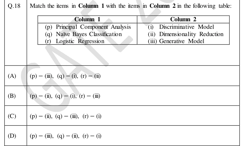
Match the items in Column 1 with the items in Column 2 in the following table:

| Column 1 | Column 2 |
|---|---|
| (p) Principal Component Analysis | (i) Discriminative Model |
| (q) Naïve Bayes Classification | (ii) Dimensionality Reduction |
| (r) Logistic Regression | (iii) Generative Model |

GATE 2024 DA question 18: A two-column table. — Figure from the GATE 2024 DA paper. It is part of the question.

(A)
(p) − (iii), (q) − (i), (r) − (ii)
(B)
(p) − (ii), (q) − (i), (r) − (iii)
(C)
(p) − (ii), (q) − (iii), (r) − (i)
(D)
(p) − (iii), (q) − (ii), (r) − (i)

Answer and solution

GATE 2024 DA Q.18: answer and solution

GATE 2024 DA Q.20

GATE 2024 · DAQ.20 · 1 mark · MCQ

Given a dataset with $K$ binary-valued attributes (where $K > 2$ ) for a two-class classification task, the number of parameters to be estimated for learning a naïve Bayes classifier is

(A)
$2^{K} + 1$
(B)
$2 K + 1$
(C)
$2^{K + 1} + 1$
(D)
$K^{2} + 1$

Answer and solution

GATE 2024 DA Q.20: answer and solution

See the question in the paper

Tap to open full size

GATE 2024 DA Q.20: answer and solution

GATE 2024 DA Q.63

GATE 2024 · DAQ.63 · 2 marks · NAT

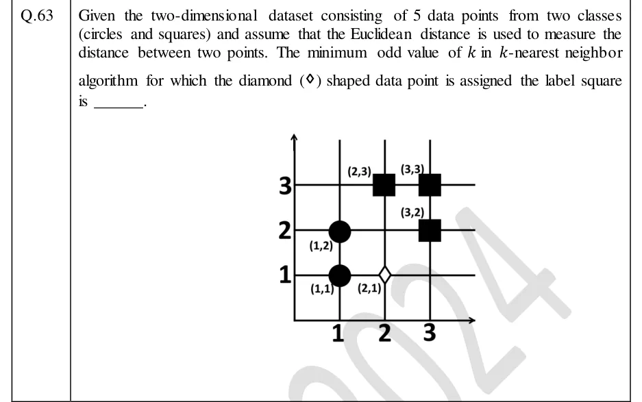
Given the two-dimensional dataset consisting of 5 data points from two classes (circles and squares) and assume that the Euclidean distance is used to measure the distance between two points. The minimum odd value of $k$ in $k$ -nearest neighbor algorithm for which the diamond ( $◊$ ) shaped data point is assigned the label square is ______.

GATE 2024 DA question 63: A 2D grid plot with x-axis and y-axis both marked 1, 2, 3. — Figure from the GATE 2024 DA paper. It is part of the question.

Answer and solution

GATE 2024 DA Q.63: answer and solution

PRACTICE

6 questions to test yourself

PRACTICE 11 mark · MCQ

A logistic regression model has weight $w_{1} = ln 3$ for feature $x_{1}$ (natural log). With all other features fixed, increasing $x_{1}$ by 1 multiplies the odds $P (y = 1 ∣ x) / P (y = 0 ∣ x)$ by a factor of

(A)
$ln 3 \approx 1.099$
(B)
3
(C)
$1/3$
(D)
$e^{3}$

Answer and solution

Answer: (B)

The log-odds equal $w^{⊤} x + b$ , so increasing $x_{1}$ by 1 adds $w_{1} = ln 3$ to the log-odds.
Adding $ln 3$ to the log of the odds multiplies the odds by $e^{l n 3} = 3$ .

PRACTICE 22 marks · NAT

A logistic regression model has $w = (1, - 1)$ and $b = 0$ . A training sample $x = (2, 1)$ has label $y = 0$ . Take the cross-entropy loss (natural log) of this single sample. Find the gradient component $\partial J / \partial w_{1}$ , correct to three decimal places.

Answer and solution

Answer: $1.462$ (accepted range $\pm 0.002$ )

$z = 1 (2) + (- 1) (1) + 0 = 1$ .
$p = σ (1) = 1/ (1 + e^{- 1}) \approx 0.7311$ .
$\partial J / \partial w_{1} = (p - y) x_{1} = (0.7311 - 0) (2) \approx 1.462$ .

PRACTICE 32 marks · NAT

Six training emails have binary features Free and Win. Rows (Free, Win, class): (Y,Y,Spam), (Y,N,Spam), (Y,Y,Spam), (N,N,Ham), (Y,N,Ham), (N,Y,Ham). A naive Bayes classifier uses Laplace smoothing with $α = 1$ on the likelihoods: add 1 to each count and 2 to each class count, since each feature has two values. The priors are estimated without smoothing. For a new email with Free = Y and Win = N, find $P (Spam ∣ Free = Y, Win = N)$ , correct to three decimal places.

Answer and solution

Answer: $0.571$ (accepted range $\pm 0.005$ )

The priors are $1/2$ and $1/2$ .
Spam: $P (Free = Y ∣ S) = (3 + 1) / (3 + 2) = 4/5$ . One Spam row has Win = N, so $P (Win = N ∣ S) = (1 + 1) /5 = 2/5$ . Score $= \frac{1}{2} \cdot \frac{4}{5} \cdot \frac{2}{5} = 0.16$ .
Ham: $P (Free = Y ∣ H) = (1 + 1) /5 = 2/5$ . Two Ham rows have Win = N, so $P (Win = N ∣ H) = (2 + 1) /5 = 3/5$ . Score $= \frac{1}{2} \cdot \frac{2}{5} \cdot \frac{3}{5} = 0.12$ .
Posterior $= 0.16/ (0.16 + 0.12) = 4/7 \approx 0.571$ .

PRACTICE 41 mark · NAT

A naive Bayes classifier has $K = 3$ classes and $d = 10$ binary features. How many independent parameters (class priors plus class-conditional feature probabilities) must it estimate?

Answer and solution

Answer: $32$

Priors: the three class probabilities sum to 1, so $K - 1 = 2$ are independent.
Likelihoods: each binary feature needs one probability $P (x_{j} = 1 ∣ c)$ per class, giving $K d = 3 \times 10 = 30$ .
Total $= 2 + 30 = 32$ . A full joint model would need $2 + 3 (2^{10} - 1) = 3071$ .

PRACTICE 52 marks · MSQ

One-dimensional training points with labels: $x = 1$ (A), $x = 2$ (A), $x = 4$ (B), $x = 5$ (B), $x = 6$ (B). A k-NN classifier (Euclidean distance, majority vote) classifies the query $x = 2.9$ . For which of the following settings is the predicted class A?

(A)
$k = 1$
(B)
$k = 3$
(C)
$k = 5$
(D)
$k = 4$ , with vote ties broken in favour of class B

Answer and solution

Answer: (A), (B)

Distances from 2.9: $x = 2 \to 0.9$ , $x = 4 \to 1.1$ , $x = 1 \to 1.9$ , $x = 5 \to 2.1$ , $x = 6 \to 3.1$ .
$k = 1$ : the nearest point is $x = 2$ (A), so A.
$k = 3$ : the nearest three are $x = 2$ (A), $x = 4$ (B) and $x = 1$ (A). Two A votes against one B, so A.
$k = 5$ : all points vote, 2 A against 3 B, so B.
$k = 4$ : adding $x = 5$ (B) gives 2 A and 2 B. The tie is broken towards B, so B.

PRACTICE 61 mark · MCQ

A 1-nearest-neighbour classifier (Euclidean distance) has two training points, $P = (1, 30)$ and $Q = (5, 10)$ . The query is $q = (0, 0)$ . Its nearest neighbour is found (i) with the raw features and (ii) after dividing the second feature of every point, including the query, by 10. The nearest neighbours in (i) and (ii) are, respectively,

(A)
$Q$ and $Q$
(B)
$Q$ and $P$
(C)
$P$ and $Q$
(D)
$P$ and $P$

Answer and solution

Answer: (B)

(i) Raw: $d (q, P) = 1 + 900 \approx 30.0$ and $d (q, Q) = 25 + 100 \approx 11.2$ , so $Q$ is nearest.
(ii) Scaled: $P = (1, 3)$ and $Q = (5, 1)$ , so $d (q, P) = 10 \approx 3.16$ and $d (q, Q) = 26 \approx 5.10$ . Now $P$ is nearest.
Scaling changes the answer: $Q$ , then $P$ .

OFFICIAL GATE 2027 SYLLABUS WORDING

Copied from the GATE 2027 syllabus; see all 2027 syllabi.

GATE DA

logistic regression, k-nearest neighbour, naive Bayes classifier

Preparing in Kolkata? IAE Academy's course for GATE DA.