GATE DA

LDA, SVMs and decision trees

Linear discriminant analysis, support vector machines and decision trees

Linear discriminant analysis, support vector machines and decision trees are three classic classifiers. LDA draws a linear boundary from the class means and a shared covariance matrix. An SVM picks the separating hyperplane with the widest margin. A decision tree splits the data greedily using impurity measures such as entropy and the Gini index. The calculations to master are a discriminant score, a margin width, a kernel value and the information gain of a split. Each is short once the formulas and conventions below are fixed.

7 previous-year questions · 7 solved · 6 practice questions

Conventions and the classification setting

All three methods learn a rule from labelled training data $(x_{i}, y_{i})$ , $i = 1, \dots, n$ . Each $x_{i} \in R^{d}$ is a feature vector, written in bold and treated as a column vector. In a data matrix $X$ the samples are the rows. Distances are Euclidean unless stated.

LDA and decision trees handle two or more classes, labelled $k = 1, \dots, K$ (or $0, 1$ for two classes).
For an SVM the two class labels are coded $y_{i} \in {+ 1, - 1}$ . This coding is what makes the constraint $y_{i} (w \cdot x_{i} + b) \geq 1$ work.
$w$ is the weight (normal) vector and $b$ is the bias (offset) of a linear boundary $w \cdot x + b = 0$ .
$lo g$ and $ln$ mean the natural logarithm unless stated. Entropy in bits uses $lo g_{2}$ , the usual choice for decision trees, and this is stated each time below.

The boundary $w \cdot x + b = 0$ is a hyperplane. The signed distance of a point $x_{0}$ from it is $\frac{w \cdot x _{0} + b}{∥ w ∥}$ , and its absolute value is the ordinary distance. This one fact drives the SVM margin.

DISTANCE OF A POINT FROM A HYPERPLANE

d (x_{0}) = \frac{∣ w \cdot x _{0} + b ∣}{∥ w ∥}

Euclidean distance from $x_{0}$ to the hyperplane $w \cdot x + b = 0$ , for $w \neq = 0$ .

Linear discriminant analysis (LDA)

LDA is a generative classifier. It models each class as a Gaussian with its own mean $μ_{k}$ and a common (shared) covariance matrix $Σ$ , and it uses class priors $π_{k}$ . Bayes' rule then gives a rule that is linear in $x$ , because the quadratic term $x^{T} Σ^{- 1} x$ is the same for every class and cancels.

LDA PARAMETER ESTIMATES (POOLED COVARIANCE)

\hat{μ}_{k} = \frac{1}{n _{k}} i : y_{i} = k \sum x_{i}, \overset{π}{^}_{k} = \frac{n _{k}}{n}, \hat{Σ} = \frac{1}{n - K} k = 1 \sum K i : y_{i} = k \sum (x_{i} - \hat{μ}_{k}) (x_{i} - \hat{μ}_{k})^{T}

Class means, priors and the pooled within-class covariance, where $n_{k}$ is the number of samples in class $k$ . Dividing by $n$ instead of $n - K$ only rescales $\hat{Σ}$ . With equal priors the decisions are unchanged. With unequal priors the $ln π_{k}$ term gets a slightly different relative weight, so borderline decisions can change.

LINEAR DISCRIMINANT FUNCTION

δ_{k} (x) = x^{T} Σ^{- 1} μ_{k} - \frac{1}{2} μ_{k}^{T} Σ^{- 1} μ_{k} + ln π_{k}

Assign $x$ to the class with the largest $δ_{k} (x)$ ; $ln$ is the natural logarithm. This assumes Gaussian classes with a common $Σ$ .

TWO-CLASS LDA RULE

w = Σ^{- 1} (μ_{1} - μ_{0}), predict class 1 if w^{T} (x - \frac{μ _{0} + μ _{1}}{2}) + ln \frac{π _{1}}{π _{0}} > 0

This is $δ_{1} (x) - δ_{0} (x) > 0$ . The boundary is a hyperplane with normal vector $Σ^{- 1} (μ_{1} - μ_{0})$ . It passes through the midpoint of the means when $π_{0} = π_{1}$ . Unequal priors shift it away from the more probable class.

With equal priors and any shared $Σ$ , LDA assigns $x$ to the class whose mean is nearest in Mahalanobis distance $(x - μ_{k})^{T} Σ^{- 1} (x - μ_{k})$ . If also $Σ = σ^{2} I$ , this becomes the nearest class mean in Euclidean distance. When $Σ$ is not a multiple of $I$ , $w$ is in general not parallel to the line joining the means, because $Σ^{- 1}$ down-weights directions of high variance. The exception is when $μ_{1} - μ_{0}$ is an eigenvector of $Σ$ ; then $w$ stays parallel to it.

EXAM TIP

A classifier with a separate covariance matrix $Σ_{k}$ for each class is quadratic discriminant analysis (QDA), not LDA. The shared covariance is exactly what makes the LDA boundary linear.

Fisher's criterion

Fisher's view is geometric and needs no Gaussian assumption. Project the data onto a direction $w$ , and choose the $w$ that pushes the projected class means far apart relative to the spread within each projected class. For two classes with sample means $μ_{0}, μ_{1}$ , define the within-class scatter $S_{W} = \sum_{k} \sum_{i \in k} (x_{i} - μ_{k}) (x_{i} - μ_{k})^{T}$ and the between-class scatter $S_{B} = (μ_{1} - μ_{0}) (μ_{1} - μ_{0})^{T}$ .

FISHER CRITERION (TWO CLASSES)

J (w) = \frac{w ^{T} S _{B} w}{w ^{T} S _{W} w} = \frac{( m _{1} - m _{0} ) ^{2}}{s _{0}^{2} + s _{1}^{2}}

Here $m_{k} = w^{T} μ_{k}$ are the projected means and $s_{k}^{2} = \sum_{i \in k} (w^{T} x_{i} - m_{k})^{2}$ the projected scatters. Maximise over $w$ . $J$ depends only on the direction of $w$ , not on its length.

FISHER'S OPTIMAL DIRECTION

w^{*} \propto S_{W}^{- 1} (μ_{1} - μ_{0})

The same direction as the two-class LDA weight vector, because $S_{W} = (n - 2) \hat{Σ}$ is proportional to the pooled covariance. $S_{W}$ must be invertible.

Fisher's method gives only a direction. To classify you still have to choose a threshold on the projection, for example the midpoint of the projected means. For $K$ classes, $S_{B}$ has rank at most $K - 1$ , so there are at most $min (K - 1, d)$ useful discriminant directions.

Worked example: LDA

WORKED EXAMPLE

Two classes in $R^{2}$ have means $μ_{0} = (0, 0)^{T}$ and $μ_{1} = (4, 2)^{T}$ and share the covariance $Σ = [4001]$ . Classify $x = (3, 1)^{T}$ (a) with equal priors, (b) with priors $π_{0} = 0.8, π_{1} = 0.2$ .

Solution

$Σ^{- 1} = [1/4 0 01]$ , so $w = Σ^{- 1} (μ_{1} - μ_{0}) = (1, 2)^{T}$ .
The midpoint of the means is $m = (2, 1)^{T}$ . Then $x - m = (1, 0)^{T}$ and $w^{T} (x - m) = 1$ .
(a) Equal priors: $ln (π_{1} / π_{0}) = 0$ , so the score is $+ 1 > 0$ and $x$ goes to class 1.
(b) $ln (0.2/0.8) = - ln 4 \approx - 1.386$ , so the score is $1 - 1.386 = - 0.386 < 0$ and $x$ goes to class 0.

Answer: (a) Class 1. (b) Class 0. The strong prior for class 0 moves the boundary towards class 1 and flips the decision.

Support vector machines: the maximum-margin hyperplane

When data is linearly separable, many hyperplanes separate the classes. The SVM picks the one with the largest margin, which is the gap between the two classes measured perpendicular to the boundary. Rescale $(w, b)$ so that the closest points of each class satisfy $w \cdot x + b = \pm 1$ ; this is the canonical scaling. The two margin hyperplanes $w \cdot x + b = + 1$ and $w \cdot x + b = - 1$ are then parallel to the boundary, and each lies at distance $1/ ∥ w ∥$ from it.

MARGIN WIDTH

margin width = \frac{2}{∥ w ∥}

The distance between the hyperplanes $w \cdot x + b = \pm 1$ . Valid only under the canonical scaling (closest points at $\pm 1$ ). The bias $b$ does not affect it.

HARD-MARGIN SVM (PRIMAL)

w, b min \frac{1}{2} ∥ w ∥^{2} subject to y_{i} (w \cdot x_{i} + b) \geq 1, i = 1, \dots, n

Requires linearly separable data. Maximising $2/ ∥ w ∥$ is the same as minimising $\frac{1}{2} ∥ w ∥^{2}$ .

HARD-MARGIN SVM (DUAL)

α max i \sum α_{i} - \frac{1}{2} i, j \sum α_{i} α_{j} y_{i} y_{j} x_{i} \cdot x_{j}, α_{i} \geq 0, i \sum α_{i} y_{i} = 0, w = i \sum α_{i} y_{i} x_{i}

Only points with $α_{i} > 0$ contribute to $w$ ; these are the support vectors. By complementary slackness, $α_{i} [y_{i} (w \cdot x_{i} + b) - 1] = 0$ , so every support vector lies exactly on $y_{i} (w \cdot x_{i} + b) = 1$ .

Every support vector lies on a margin hyperplane. Removing a point with $α_{i} = 0$ and retraining leaves the solution unchanged. In degenerate cases a point can lie on a margin hyperplane and still have $α_{i} = 0$ .
The decision function is $f (x) = sign (\sum_{i} α_{i} y_{i} x_{i} \cdot x + b)$ .
$b$ can be found from any support vector $x_{s}$ : $b = y_{s} - w \cdot x_{s}$ (because $y_{s} = \pm 1$ ).
Because $\sum_{i} α_{i} y_{i} = 0$ , the $α$ values of the positive support vectors add up to those of the negative ones.
At the hard-margin optimum $∥ w ∥^{2} = \sum_{i} α_{i}$ , so the margin width is also $2/ \sum_{i} α_{i}$ .

WORKED EXAMPLE

Training data: positives $(2, 2), (3, 3)$ and negatives $(0, 0), (- 1, - 1)$ . Find the hard-margin hyperplane and its margin width.

Solution

All four points lie on the line $x_{1} = x_{2}$ . The closest points of the two classes are $(2, 2)$ and $(0, 0)$ , at distance $22$ . The maximum-margin boundary is the perpendicular bisector of the segment joining them, so $w = a (1, 1)$ for some $a > 0$ .
Both closest points are support vectors, so their constraints are active. For $(0, 0)$ with $y = - 1$ : $- (w \cdot 0 + b) = 1$ , so $b = - 1$ . For $(2, 2)$ with $y = + 1$ : $2 a + 2 a + b = 1$ , so $4 a = 2$ , $a = \frac{1}{2}$ and $w = (0.5, 0.5)$ .
$∥ w ∥ = 0.5 \approx 0.7071$ , so the margin width is $2/0.7071 \approx 2.83 = 22$ . This equals the distance between the closest points, as it should.
Check the other points. For $(3, 3)$ : $w \cdot x + b = 1.5 + 1.5 - 1 = 2$ , so $y (w \cdot x + b) = 2 \geq 1$ . For $(- 1, - 1)$ : $w \cdot x + b = - 0.5 - 0.5 - 1 = - 2$ , so $y (w \cdot x + b) = (- 1) (- 2) = 2 \geq 1$ . Both lie outside the margin and have $α_{i} = 0$ .
Dual check: $w = α_{1} (2, 2) - α_{2} (0, 0) = (0.5, 0.5)$ gives $α_{1} = \frac{1}{4}$ . Then $\sum_{i} α_{i} y_{i} = 0$ gives $α_{2} = \frac{1}{4}$ , and $\sum_{i} α_{i} = \frac{1}{2} = ∥ w ∥^{2}$ , as it must.

Answer: The hyperplane is $0.5 x_{1} + 0.5 x_{2} - 1 = 0$ , i.e. $x_{1} + x_{2} = 2$ . The margin width is $22 \approx 2.83$ . The support vectors are $(2, 2)$ and $(0, 0)$ , each with $α = \frac{1}{4}$ .

Soft margins, the role of C, and kernels

Real data is rarely separable. The soft-margin SVM lets points violate the margin by a slack $ξ_{i} \geq 0$ and charges a penalty for it. The parameter $C > 0$ trades margin width against violations. For finite $C$ the problem has a solution whether or not the data is separable.

SOFT-MARGIN SVM (PRIMAL)

w, b, ξ min \frac{1}{2} ∥ w ∥^{2} + C i = 1 \sum n ξ_{i} s.t. y_{i} (w \cdot x_{i} + b) \geq 1 - ξ_{i}, ξ_{i} \geq 0

In the dual, the only change from the hard margin is the box constraint $0 \leq α_{i} \leq C$ .

SOFT-MARGIN SVM AS HINGE LOSS

w, b min \frac{1}{2} ∥ w ∥^{2} + C i = 1 \sum n max (0, 1 - y_{i} (w \cdot x_{i} + b))

At the optimum $ξ_{i} = max (0, 1 - y_{i} (w \cdot x_{i} + b))$ , which turns the constrained problem into this unconstrained one.

Multiplier / slack	Where the point lies
$α_{i} = 0$ ( $ξ_{i} = 0$ )	Correct side, on or outside the margin; not a support vector
$0 < α_{i} < C, ξ_{i} = 0$	Exactly on the margin; a support vector
$α_{i} = C, 0 < ξ_{i} < 1$	Inside the margin but on the correct side; a support vector
$α_{i} = C, ξ_{i} = 1$	On the decision boundary $w \cdot x + b = 0$ ; a support vector
$α_{i} = C, ξ_{i} > 1$	Misclassified; a support vector

Each misclassified training point has $ξ_{i} > 1$ , so $\sum_{i} ξ_{i}$ is an upper bound on the number of training errors.
In the soft-margin case, compute $b = y_{s} - w \cdot x_{s}$ from a support vector with $0 < α_{s} < C$ , which lies exactly on the margin.

	Large $C$	Small $C$
Penalty on violations	Heavy	Light
Margin	Tends to be narrower	Tends to be wider
Training errors	Tend to be fewer; approaches the hard margin as $C \to \infty$ on separable data	More are tolerated
Risk	Overfitting, sensitivity to outliers	Underfitting

A kernel lets the SVM draw a non-linear boundary. Replace every dot product $x_{i} \cdot x_{j}$ by $K (x_{i}, x_{j}) = ϕ (x_{i}) \cdot ϕ (x_{j})$ , where $ϕ$ maps into a higher-dimensional feature space. The mapping $ϕ$ never has to be computed. $K$ must be symmetric, and its Gram matrix $[K (x_{i}, x_{j})]$ must be positive semi-definite (no negative eigenvalues) for every finite set of points.

COMMON KERNELS

K_{lin} (x, z) = x \cdot z, K_{poly} (x, z) = (x \cdot z + c)^{p}, K_{RBF} (x, z) = exp (- γ ∥ x - z ∥^{2})

Polynomial kernel: degree $p$ a positive integer and $c \geq 0$ . RBF (Gaussian) kernel: $γ > 0$ , often written $γ = 1/ (2 σ^{2})$ . RBF values lie in $(0, 1]$ and equal 1 only when $x = z$ .

KERNELISED DECISION FUNCTION

f (x) = sign (i \sum α_{i} y_{i} K (x_{i}, x) + b)

Only the support vectors ( $α_{i} > 0$ ) contribute to the sum.

EXAM TIP

For the polynomial kernel $(x \cdot z + 1)^{2}$ in two dimensions, the implicit feature space has 6 dimensions: $1, 2 x_{1}, 2 x_{2}, x_{1}^{2}, x_{2}^{2}, 2 x_{1} x_{2}$ . In general $(x \cdot z + c)^{p}$ with $c > 0$ in $d$ dimensions corresponds to $(p d + p)$ features, and $(2 4) = 6$ here. A very large RBF $γ$ makes each training point its own island and tends to overfit. A very small $γ$ gives a very smooth boundary, close to linear.

Decision trees: impurity, information gain and the split

A decision tree classifies by asking a sequence of questions about the features. Each internal node tests one feature; for a numeric feature the test is a threshold such as $x_{j} \leq t$ . Each leaf predicts the majority class of the training samples that reach it. The tree is grown greedily from the root: at each node, try the candidate splits, keep the one that makes the children purest, then recurse. There is no backtracking, so greedy growth is not guaranteed to give the best or the smallest tree. Depth is counted with the root at depth 0.

ENTROPY (IN BITS)

H (S) = - k = 1 \sum K p_{k} lo g_{2} p_{k}, 0 lo g_{2} 0 := 0

$p_{k}$ is the fraction of class $k$ in node $S$ . Entropy ranges from $0$ (a pure node) to $lo g_{2} K$ (all classes equally likely), which is $1$ bit for two balanced classes.

GINI INDEX

G (S) = 1 - k = 1 \sum K p_{k}^{2}

Ranges from $0$ (pure) to $1 - 1/ K$ (equal classes), which is $0.5$ for two balanced classes. For two classes with proportions $p, 1 - p$ : $G = 2 p (1 - p)$ .

MISCLASSIFICATION ERROR

E (S) = 1 - k max p_{k}

Ranges from $0$ to $1 - 1/ K$ . For two classes, $E = min (p, 1 - p)$ . Entropy and Gini respond more strongly to changes in node purity, so they are the usual criteria for growing a tree.

INFORMATION GAIN OF A SPLIT

IG (S, A) = H (S) - v \sum \frac{∣ S _{v} ∣}{∣ S ∣} H (S_{v})

$S_{v}$ is the subset sent to child $v$ by the test $A$ . The same weighted-average pattern with $G$ in place of $H$ gives the Gini reduction. Choose the split with the largest gain.

GAIN RATIO

GainRatio (S, A) = \frac{IG ( S , A )}{SplitInfo ( S , A )}, SplitInfo (S, A) = - v \sum \frac{∣ S _{v} ∣}{∣ S ∣} lo g_{2} \frac{∣ S _{v} ∣}{∣ S ∣}

Divides the gain by the entropy (in bits) of the split proportions themselves. This penalises tests that break the node into many small branches.

Compute the class counts at the node and its impurity.
For each candidate split, count the classes in every child and compute each child's impurity.
Weight each child's impurity by its share of the samples and add the results.
Gain = parent impurity minus weighted child impurity. Pick the split with the largest gain.
For a numeric feature, sort the values. It is enough to test thresholds midway between neighbouring distinct values whose labels differ.

WORKED EXAMPLE

A node has 10 samples: 6 positive and 4 negative. A test $A$ sends 5 samples left (4 positive, 1 negative) and 5 right (2 positive, 3 negative). Find the information gain (in bits) and the Gini reduction.

Solution

Parent: $H = - 0.6 lo g_{2} 0.6 - 0.4 lo g_{2} 0.4 \approx 0.4422 + 0.5288 = 0.9710$ .
Left: $p = (0.8, 0.2)$ , $H \approx 0.2575 + 0.4644 = 0.7219$ . Right: $p = (0.4, 0.6)$ , $H = 0.9710$ .
Weighted child entropy: $0.5 (0.7219) + 0.5 (0.9710) = 0.8464$ . So IG $= 0.9710 - 0.8464 \approx 0.125$ bits.
Gini: parent $1 - 0.36 - 0.16 = 0.48$ ; left $1 - 0.64 - 0.04 = 0.32$ ; right $1 - 0.16 - 0.36 = 0.48$ . Weighted $= 0.5 (0.32) + 0.5 (0.48) = 0.40$ , so the reduction is $0.48 - 0.40 = 0.08$ .

Answer: Information gain $\approx 0.125$ bits; Gini reduction $= 0.08$ .

EXAM TIP

Information gain is never negative, because entropy is concave: the weighted child entropy cannot exceed the parent's. A gain of exactly 0 means every child has the same class proportions as the parent. Plain information gain favours features with many distinct values; an ID-like feature gives pure single-sample children and the maximum possible gain. Gain ratio is the usual remedy.

Depth, pruning, overfitting and comparison

A tree grown until every leaf is pure fits the training set perfectly, provided no two identical inputs carry different labels. Such a tree usually overfits: low training error, higher test error. Depth and number of leaves measure complexity. With the root at depth 0, a tree of depth $D$ has at most $2^{D}$ leaves if every split is binary.

Pre-pruning (early stopping): stop growing at a maximum depth, at a minimum number of samples per node, or when the best gain falls below a threshold.
Post-pruning: grow the full tree, then cut back subtrees whose removal does not hurt error on a held-out validation set. Alternatively, use a complexity penalty: cost-complexity pruning trades training error against the number of leaves.
Deeper trees tend to have lower bias and higher variance; shallow trees tend to the reverse.

Property	LDA	SVM	Decision tree
Boundary	Linear (shared $Σ$ )	Linear, or non-linear via a kernel	Axis-parallel splits; predictions piecewise constant
Objective	Class-conditional Gaussians; Fisher separation	Maximum margin plus a slack penalty	Greedy impurity reduction
Key hyper-parameters	None essential (priors can be estimated or set)	$C$ , the kernel and its parameters	Depth, minimum samples per node, pruning
Depends on	All training points, through the means and $Σ$	Support vectors only	The samples reaching each node
Does feature scaling matter?	No: any invertible linear rescaling of the features leaves the decisions unchanged	Yes, for linear and kernel SVMs alike (the margin is a Euclidean distance)	No: rescaling a feature monotonically keeps the order of its values, which is all a split uses

EXAM TIP

SVM and LDA trained on the same two-class data generally give different boundaries. LDA uses every point, through the class means and $Σ$ , while the SVM is decided by the points on or inside the margin. Moving a point that stays on the correct side, outside the margin, changes the class mean and so the LDA boundary, but it does not change the SVM.

PREVIOUS-YEAR QUESTIONS

7 questions from the DA papers

Try each question first, then open the answer. We placed each question under a topic ourselves; the exam paper does not label topics.

See these papers in full: GATE DA 2026 · GATE DA 2025 · GATE DA 2024

GATE 2026 DA Q.23

GATE 2026 · DAQ.23 · 1 mark · MSQ

In the following table, the Task column lists a few tasks related to machine learning. The Algorithm column lists a few algorithms.

Each entry "t" from the Task column is to be matched with an appropriate entry "a" from the Algorithm column such that the task "t" can be solved using the algorithm "a". Denote such a match as t:a.

| Task | Algorithm |
|---|---|
| T1 – Clustering | A1 – Markov Chain Monte Carlo |
| T2 – Classification | A2 – K-Medoid |
| T3 – Sampling | A3 – Linear Discriminant Analysis |
| T4 – Feature Extraction | A4 – Naive Bayes |

Which of the following options is/are the correct matching(s)?

(A)
T1:A4, T2:A3, T3:A1, T4:A2
(B)
T1:A2, T2:A4, T3:A1, T4:A3
(C)
T1:A3, T2:A4, T3:A1, T4:A2
(D)
T1:A4, T2:A2, T3:A1, T4:A3

Answer and solution

GATE 2026 DA Q.23: answer and solution

See the question in the paper

Tap to open full size

GATE 2026 DA Q.23: answer and solution

GATE 2025 DA Q.53

GATE 2025 · DAQ.53 · 2 marks · MSQ

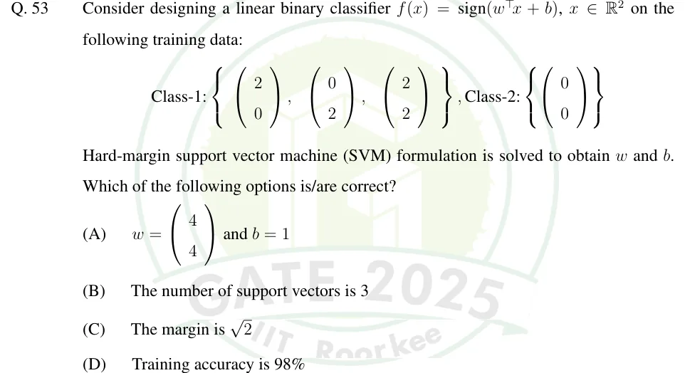
Consider designing a linear binary classifier $f (x) = sign (w^{⊤} x + b)$ , $x \in R^{2}$ on the following training data: Class-1: ${(2, 0)^{⊤}, (0, 2)^{⊤}, (2, 2)^{⊤}}$ , Class-2: ${(0, 0)^{⊤}}$ . Hard-margin support vector machine (SVM) formulation is solved to obtain $w$ and $b$ . Which of the following options is/are correct?

(A)
$w = (4, 4)^{⊤}$ and $b = 1$
(B)
The number of support vectors is 3
(C)
The margin is $2$
(D)
Training accuracy is 98%

Answer and solution

GATE 2025 DA Q.53: answer and solution

See the question in the paper

Tap to open full size

GATE 2025 DA Q.53: answer and solution

GATE 2025 DA Q.55

GATE 2025 · DAQ.55 · 2 marks · MSQ

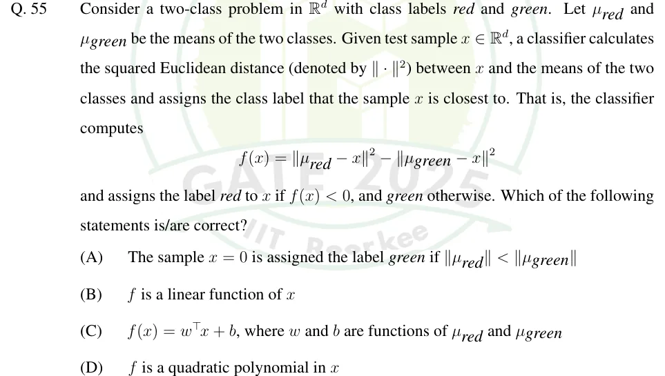
Consider a two-class problem in $R^{d}$ with class labels red and green. Let $μ_{r e d}$ and $μ_{g r ee n}$ be the means of the two classes. Given test sample $x \in R^{d}$ , a classifier calculates the squared Euclidean distance (denoted by $∥ \cdot ∥^{2}$ ) between $x$ and the means of the two classes and assigns the class label that the sample $x$ is closest to. That is, the classifier computes $f (x) = ∥ μ_{r e d} - x ∥^{2} - ∥ μ_{g r ee n} - x ∥^{2}$ and assigns the label red to $x$ if $f (x) < 0$ , and green otherwise. Which of the following statements is/are correct?

(A)
The sample $x = 0$ is assigned the label green if $∥ μ_{r e d} ∥ < ∥ μ_{g r ee n} ∥$
(B)
$f$ is a linear function of $x$
(C)
$f (x) = w^{⊤} x + b$ , where $w$ and $b$ are functions of $μ_{r e d}$ and $μ_{g r ee n}$
(D)
$f$ is a quadratic polynomial in $x$

Answer and solution

GATE 2025 DA Q.55: answer and solution

See the question in the paper

Tap to open full size

GATE 2025 DA Q.55: answer and solution

GATE 2024 DA Q.17

GATE 2024 · DAQ.17 · 1 mark · MCQ

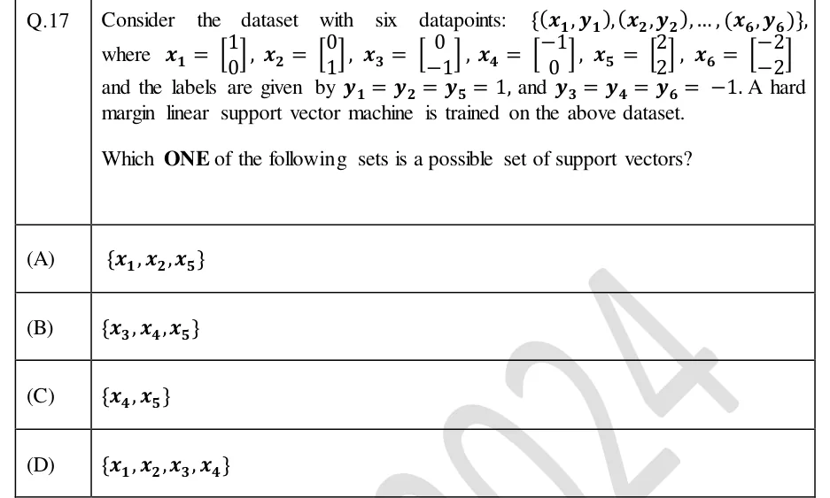
Consider the dataset with six datapoints: ${(x_{1}, y_{1}), (x_{2}, y_{2}), \dots, (x_{6}, y_{6})}$ , where $x_{1} = [10]$ , $x_{2} = [01]$ , $x_{3} = [0 - 1]$ , $x_{4} = [- 1 0]$ , $x_{5} = [22]$ , $x_{6} = [- 2 - 2]$ and the labels are given by $y_{1} = y_{2} = y_{5} = 1$ , and $y_{3} = y_{4} = y_{6} = - 1$ . A hard margin linear support vector machine is trained on the above dataset. Which ONE of the following sets is a possible set of support vectors?

(A)
${x_{1}, x_{2}, x_{5}}$
(B)
${x_{3}, x_{4}, x_{5}}$
(C)
${x_{4}, x_{5}}$
(D)
${x_{1}, x_{2}, x_{3}, x_{4}}$

Answer and solution

GATE 2024 DA Q.17: answer and solution

See the question in the paper

Tap to open full size

GATE 2024 DA Q.17: answer and solution

GATE 2024 DA Q.22

GATE 2024 · DAQ.22 · 1 mark · MCQ

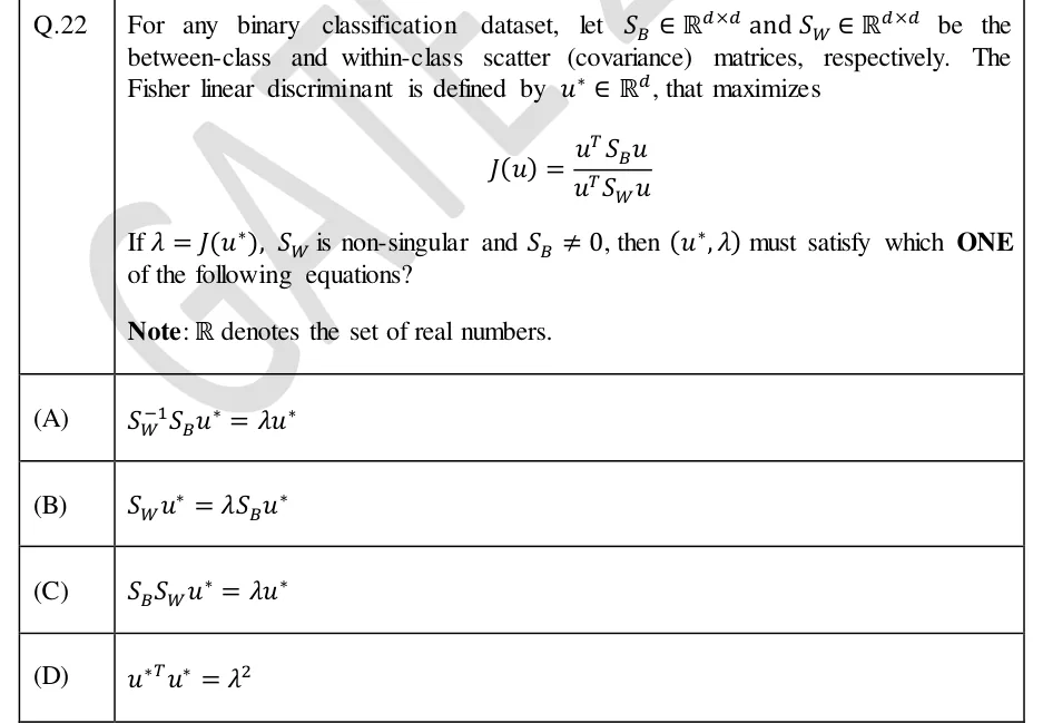
For any binary classification dataset, let $S_{B} \in R^{d \times d}$ and $S_{W} \in R^{d \times d}$ be the between-class and within-class scatter (covariance) matrices, respectively. The Fisher linear discriminant is defined by $u^{*} \in R^{d}$ , that maximizes

J (u) = \frac{u ^{T} S _{B} u}{u ^{T} S _{W} u}

If $λ = J (u^{*})$ , $S_{W}$ is non-singular and $S_{B} \neq = 0$ , then $(u^{*}, λ)$ must satisfy which ONE of the following equations?

Note: $R$ denotes the set of real numbers.

(A)
$S_{W}^{- 1} S_{B} u^{*} = λ u^{*}$
(B)
$S_{W} u^{*} = λ S_{B} u^{*}$
(C)
$S_{B} S_{W} u^{*} = λ u^{*}$
(D)
$u^{* T} u^{*} = λ^{2}$

Answer and solution

GATE 2024 DA Q.22: answer and solution

See the question in the paper

Tap to open full size

GATE 2024 DA Q.22: answer and solution

GATE 2024 DA Q.53

GATE 2024 · DAQ.53 · 2 marks · MSQ

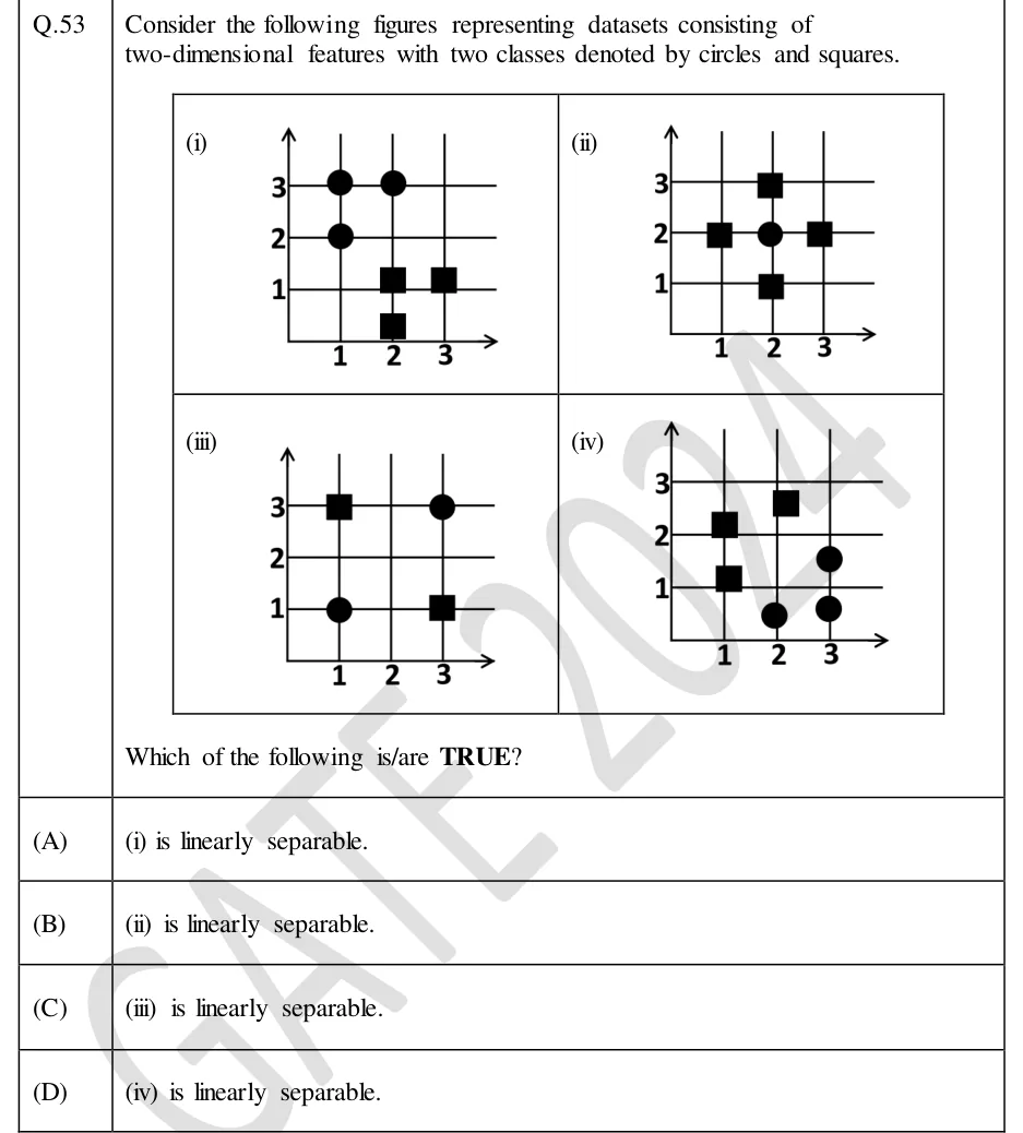
Consider the following figures representing datasets consisting of two-dimensional features with two classes denoted by circles and squares. Which of the following is/are TRUE?

GATE 2024 DA question 53: Four panels, each a 2-D scatter on axes with ticks 1, 2, 3 (both axes). — Figure from the GATE 2024 DA paper. It is part of the question.

(A)
(i) is linearly separable.
(B)
(ii) is linearly separable.
(C)
(iii) is linearly separable.
(D)
(iv) is linearly separable.

Answer and solution

GATE 2024 DA Q.53: answer and solution

GATE 2024 DA Q.62

GATE 2024 · DAQ.62 · 2 marks · NAT

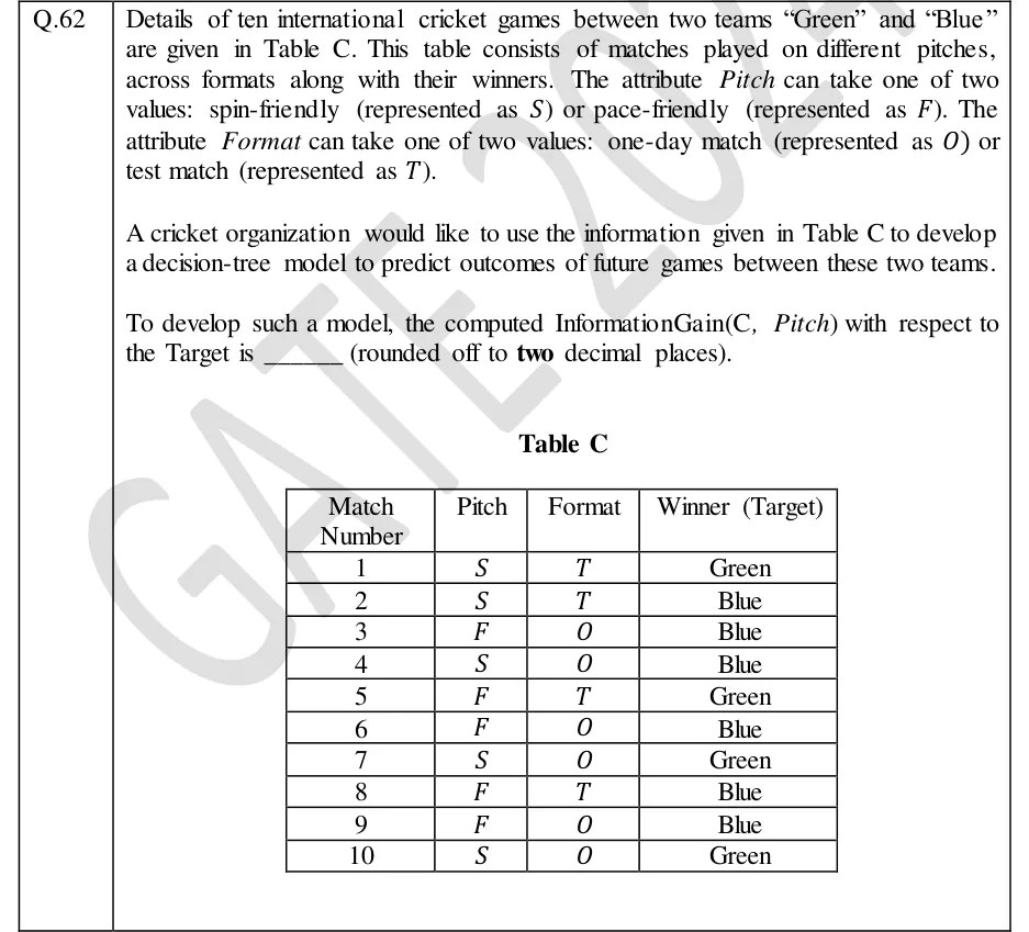
Details of ten international cricket games between two teams "Green" and "Blue" are given in Table C. This table consists of matches played on different pitches, across formats along with their winners. The attribute Pitch can take one of two values: spin-friendly (represented as S) or pace-friendly (represented as F). The attribute Format can take one of two values: one-day match (represented as O) or test match (represented as T).

A cricket organization would like to use the information given in Table C to develop a decision-tree model to predict outcomes of future games between these two teams.

To develop such a model, the computed InformationGain(C, Pitch) with respect to the Target is ______ (rounded off to two decimal places).

GATE 2024 DA question 62: Table C with columns Match Number, Pitch, Format, Winner (Target). — Figure from the GATE 2024 DA paper. It is part of the question.

Answer and solution

GATE 2024 DA Q.62: answer and solution

PRACTICE

6 questions to test yourself

PRACTICE 11 mark · NAT

A hard-margin linear SVM trained on separable data gives $w = (3, 4)^{T}$ and $b = - 2$ under the canonical scaling (support vectors satisfy $y_{i} (w \cdot x_{i} + b) = 1$ ). What is the width of the margin, $2/ ∥ w ∥$ ? Give your answer to one decimal place.

Answer and solution

Answer: $0.4$ (accepted range $\pm 0.01$ )

$∥ w ∥ = 3^{2} + 4^{2} = 5$ .
Margin width $= 2/5 = 0.4$ . The bias $b$ does not affect the width.

PRACTICE 21 mark · MCQ

A decision-tree node holds 8 samples: 2 of class A, 2 of class B and 4 of class C. Using $lo g_{2}$ , the entropy of the node in bits is:

(A)
1
(B)
1.5
(C)
1.585
(D)
2

Answer and solution

Answer: (B)

The proportions are $0.25, 0.25, 0.5$ .
$H = - 0.25 lo g_{2} 0.25 - 0.25 lo g_{2} 0.25 - 0.5 lo g_{2} 0.5 = 0.25 \cdot 2 + 0.25 \cdot 2 + 0.5 \cdot 1 = 1.5$ bits.
The maximum for three classes is $lo g_{2} 3 \approx 1.585$ , reached only when the classes are equal. This node is not balanced, so its entropy is below that.

PRACTICE 32 marks · MSQ

Which of the following statements about the soft-margin SVM with penalty parameter $C$ are correct?

(A)
A very small $C$ tolerates many margin violations and favours a wider margin.
(B)
As $C \to \infty$ on linearly separable data, the solution approaches the hard-margin SVM.
(C)
Every training point with $α_{i} = 0$ is a support vector.
(D)
Decreasing $C$ always lowers the training error.

Answer and solution

Answer: (A), (B)

A is true. A small $C$ makes slack cheap, so the $\frac{1}{2} ∥ w ∥^{2}$ term dominates and the margin widens.
B is true. A huge $C$ makes any violation prohibitively expensive, which gives the hard-margin problem when a separating hyperplane exists.
C is false. Support vectors are exactly the points with $α_{i} > 0$ .
D is false. Decreasing $C$ tolerates more violations, so training error generally rises or stays the same.

PRACTICE 42 marks · NAT

A node has 12 samples: 8 positive and 4 negative. A split sends 6 samples to the left child (all positive) and 6 to the right child (2 positive, 4 negative). Using the Gini index, find the reduction in impurity (parent Gini minus weighted child Gini). Give the answer to three decimal places.

Answer and solution

Answer: $0.222$ (accepted range $\pm 0.005$ )

Parent: $p = (2/3, 1/3)$ , so $G = 1 - 4/9 - 1/9 = 4/9 \approx 0.4444$ .
The left child is pure, so $G = 0$ . Right child: $p = (1/3, 2/3)$ , so $G = 1 - 1/9 - 4/9 = 4/9$ .
Weighted child Gini $= \frac{1}{2} \cdot 0 + \frac{1}{2} \cdot \frac{4}{9} = \frac{2}{9} \approx 0.2222$ .
Reduction $= \frac{4}{9} - \frac{2}{9} = \frac{2}{9} \approx 0.222$ .

PRACTICE 51 mark · NAT

For the RBF kernel $K (x, z) = exp (- γ ∥ x - z ∥^{2})$ with $γ = 0.5$ , compute $K (x, z)$ for $x = (1, 2)^{T}$ and $z = (2, 0)^{T}$ , where $∥ \cdot ∥$ is the Euclidean norm. Give the answer to three decimal places.

Answer and solution

Answer: $0.082$ (accepted range $\pm 0.001$ )

$x - z = (- 1, 2)^{T}$ , so $∥ x - z ∥^{2} = 1 + 4 = 5$ .
$K = exp (- 0.5 \times 5) = e^{- 2.5} \approx 0.0821$ .
Check: the value lies in $(0, 1]$ , as every RBF kernel value must.

PRACTICE 62 marks · MCQ

Two classes share the covariance matrix $Σ = [1004]$ , with means $μ_{0} = (1, 0)^{T}$ and $μ_{1} = (3, 2)^{T}$ and equal priors. With $w = Σ^{- 1} (μ_{1} - μ_{0})$ and $m$ the midpoint of the means, the LDA rule assigns the point $x = (1, 3)^{T}$ to:

(A)
Class 0, since $w^{T} (x - m) = - 1$
(B)
Class 1, since $w^{T} (x - m) = + 2$
(C)
Class 1, since $w^{T} (x - m) = + 1$
(D)
Class 0, since $w^{T} (x - m) = - 2$

Answer and solution

Answer: (A)

$Σ^{- 1} = diag (1, 1/4)$ and $μ_{1} - μ_{0} = (2, 2)^{T}$ , so $w = (2, 0.5)^{T}$ .
The midpoint is $m = (2, 1)^{T}$ , so $x - m = (- 1, 2)^{T}$ .
$w^{T} (x - m) = 2 (- 1) + 0.5 (2) = - 1 < 0$ . With equal priors the point goes to class 0.
With $Σ = I$ the score would be $2 (- 1) + 2 (2) = + 2$ and the answer would flip, which shows why $Σ^{- 1}$ matters.

OFFICIAL GATE 2027 SYLLABUS WORDING

Copied from the GATE 2027 syllabus; see all 2027 syllabi.

GATE DA

linear discriminant analysis, support vector machine, decision trees

Preparing in Kolkata? IAE Academy's course for GATE DA.