IAE Academy

GATE BT

Bioinformatics

Databases, sequence alignment, phylogeny and structure prediction

Bioinformatics turns raw sequence and structure data into biological insight. These notes cover which database or search tool holds what, how sequence alignments are scored and computed (substitution matrices, gap penalties, dynamic programming, BLAST statistics), how phylogenetic trees are built and read, how genes, functions and protein structures are predicted, and how the -omics layers (genomics, transcriptomics, proteomics, metabolomics, metagenomics) feed systems biology and metabolic engineering.

11 previous-year questions · 10 solved · 7 practice questions

Biological databases and search tools

Biological databases are grouped by how their data is produced. Primary databases hold experimentally derived data as submitted, such as nucleotide sequences. Secondary databases hold information derived from primary data, such as motifs, domain families and conserved patterns built from alignments. Composite databases merge several primary sources into one non-redundant set, for example the non-redundant protein set searched by BLAST. Structural databases (atomic coordinates) and specialised databases (one organism, disease or pathway) form further groups. Three primary nucleotide databases make up the INSDC (International Nucleotide Sequence Database Collaboration): GenBank (NCBI, USA), ENA (the European Nucleotide Archive at EMBL-EBI, which holds the former EMBL-Bank) and DDBJ (Japan). They exchange new data daily, so a record carries the same accession number in all three.

Major databases and what they hold

Resource

Type

Primary content

GenBank / ENA (EMBL) / DDBJ

Primary nucleotide

Nucleotide sequences with annotation, as submitted by researchers; mirrored across the INSDC

UniProtKB (Swiss-Prot + TrEMBL)

Protein sequence knowledgebase

Protein sequences and functional annotation; Swiss-Prot entries are manually reviewed, TrEMBL entries are computationally annotated and unreviewed

PDB (Protein Data Bank)

Structural

3-D atomic coordinates of proteins and nucleic acids determined by X-ray crystallography, NMR or cryo-EM

PROSITE

Secondary

Protein sites and motifs written as patterns (regular expressions) and profiles

Pfam

Secondary

Protein domain families, each built from a multiple alignment and represented as a profile HMM

InterPro

Secondary (integrated)

Combines protein signatures from several member databases (including Pfam and PROSITE) into single entries

SCOP / CATH

Structural classification

Hierarchical classification of protein domains by structure (class, fold/architecture, superfamily, family)

KEGG

Pathway / integrated

Metabolic and signalling pathway maps linked to genes, enzymes and compounds

OMIM

Specialised

Human genes and genetic disorders/phenotypes

PubMed

Literature (bibliographic)

Citations and abstracts of biomedical literature

Search tool vs database: a key distinction

  1. A database stores records (sequences, structures, annotations). A search tool queries a database for matches to your input. BLAST searches sequence databases by sequence similarity; DALI and CE compare a 3-D structure against the PDB to find similar folds.

  2. A text/keyword search retrieves records by annotation fields (organism, gene name, accession number). A sequence-similarity search (BLAST, FASTA) retrieves records by the sequence content itself.

  3. An integrated retrieval system such as NCBI Entrez lets one query search many linked databases (nucleotide, protein, structure, literature) and follow cross-links between them. Do not confuse this with a composite database, which is a merged data set.

EXAM TIP

An accession number is shared across GenBank, ENA and DDBJ because the INSDC exchanges data. In UniProtKB each entry sits in exactly one section: Swiss-Prot (reviewed) or TrEMBL (unreviewed). A TrEMBL entry moves to Swiss-Prot once it has been manually curated. 'Unreviewed' describes the annotation, not the reliability of the sequence itself.

Sequence file formats, scoring matrices and gap penalties

Sequence and structure file formats

  1. FASTA: each record starts with a single header line beginning with > followed by an identifier and an optional description. Every following line, up to the next >, is sequence written in IUPAC one-letter codes (A, C, G, T/U plus ambiguity codes such as N for nucleotides; the 20 one-letter amino-acid codes for proteins).

  2. FASTQ (raw sequencing reads): four lines per record. Line 1 is the @ header, line 2 the sequence, line 3 a + (optionally followed by the header again), and line 4 a quality string with exactly one character per base. The per-base quality line is what FASTA lacks.

  3. GenBank flat file: a human-readable record with labelled fields (LOCUS, DEFINITION, ACCESSION, VERSION, SOURCE/ORGANISM, FEATURES with CDS and gene coordinates). The sequence follows the ORIGIN line and the record ends with //.

  4. PDB format: a structure file in which each atom is one ATOM line (standard residues) or HETATM line (ligands, water, non-standard residues), giving atom name, residue, chain and x, y, z coordinates in ångström.

PHRED BASE-QUALITY SCORE (FASTQ)

is the probability that the base call is wrong. Q = 20 means (1 error in 100, 99% accuracy); Q = 30 means (1 in 1000, 99.9%). In the common Phred+33 encoding, the quality character's ASCII code equals Q + 33.

A substitution (scoring) matrix gives a score to every possible pair of residues. The score reflects how often that substitution is seen in real alignments of related proteins, compared with how often it would occur by chance. PAM (Point Accepted Mutation) matrices start from alignments of closely related proteins. PAM1 is estimated from these alignments, and more divergent matrices are extrapolated by multiplying PAM1 by itself. BLOSUM (BLOcks SUbstitution Matrix) matrices are counted directly from ungapped conserved blocks of related proteins, with no extrapolation. For BLOSUM*n*, sequences sharing at least n% identity are clustered and counted as one, so BLOSUM62 comes from blocks clustered at 62% identity.

PAM vs BLOSUM

Property

PAM

BLOSUM

Derived from

Alignments of closely related proteins; higher matrices extrapolated from PAM1

Ungapped conserved blocks, counted directly at a stated clustering identity

What the number means

Evolutionary distance: a higher number means MORE divergence (PAM250 suits distant proteins; PAM1 corresponds to about 99% identity)

Clustering identity threshold: a higher number suits MORE similar sequences (BLOSUM80 for close sequences, BLOSUM45 for distant ones)

Approximate equivalence

PAM250

roughly comparable to BLOSUM45 (approximate only)

Common default

PAM250 for distant comparisons

BLOSUM62, the default matrix for protein BLAST (blastp)

PAM UNIT AND THE PAM SERIES

PAM1 describes a distance at which 1% of residues have changed. Higher PAM matrices are matrix powers of the PAM1 mutation-probability matrix: extrapolation, not new data. Because a site can change more than once, PAM250 does not mean 250% different; sequences at this distance still share roughly 20% identity.

LOG-ODDS SUBSTITUTION SCORE

= observed frequency of residues a and b aligned in related sequences; , = background frequencies of each residue; = scaling constant (values are then rounded to integers). A positive score means the pair occurs more often than chance (a conservative or likely substitution), zero means as often as chance, and a negative score means less often than chance.

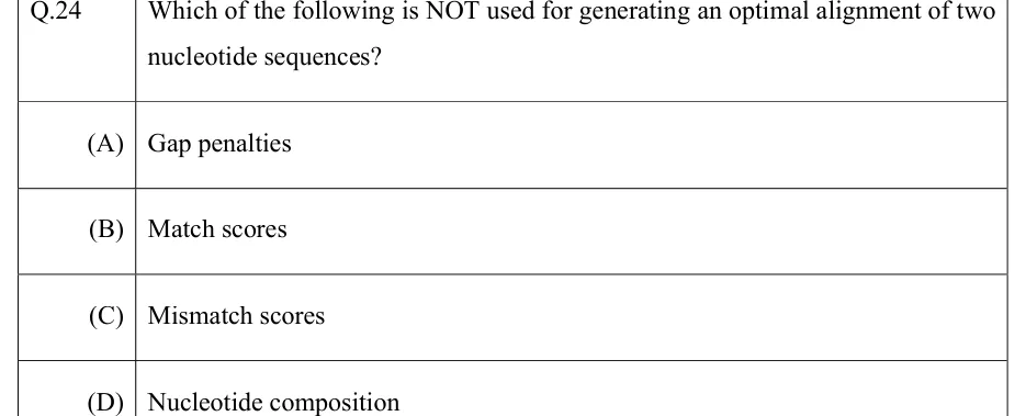
Alignments use gaps to represent insertions and deletions (indels). A linear gap penalty charges the same cost for every gap position: . An affine gap penalty, used by most practical aligners, charges more to open a gap than to extend it. The reason is that a single indel event can insert or delete several residues at once, so one long gap is biologically more plausible than several short ones of the same total length.

AFFINE GAP PENALTY

g = gap length; α = gap-opening penalty (the cost of the first gap position); β = gap-extension penalty (the cost of each further position), with α > β. Convention: some programs write the same idea as , where the opening cost is charged on top of a per-position cost for every position. Always check which form a question uses.

Pairwise sequence alignment: global, local, and BLAST

Terms to keep distinct

  1. Identity: the percentage of aligned positions with identical residues. Similarity: the percentage with identical or conservatively substituted residues (a positive score in the matrix). Both are measured quantities.

  2. Homology means shared ancestry. It is either true or false, so 'percent homology' is incorrect usage. High similarity is evidence of homology; it is not the definition.

  3. Orthologs are homologous genes separated by a speciation event (the same gene in different species). Paralogs are homologous genes separated by a gene duplication within a lineage.

  4. Dot plot: one sequence runs along each axis, and a dot marks each matching position (or window). A long main diagonal shows extended similarity. Parallel off-diagonal lines show repeats. Lines running perpendicular to the main diagonal show inverted repeats (palindromic regions when a sequence is plotted against itself).

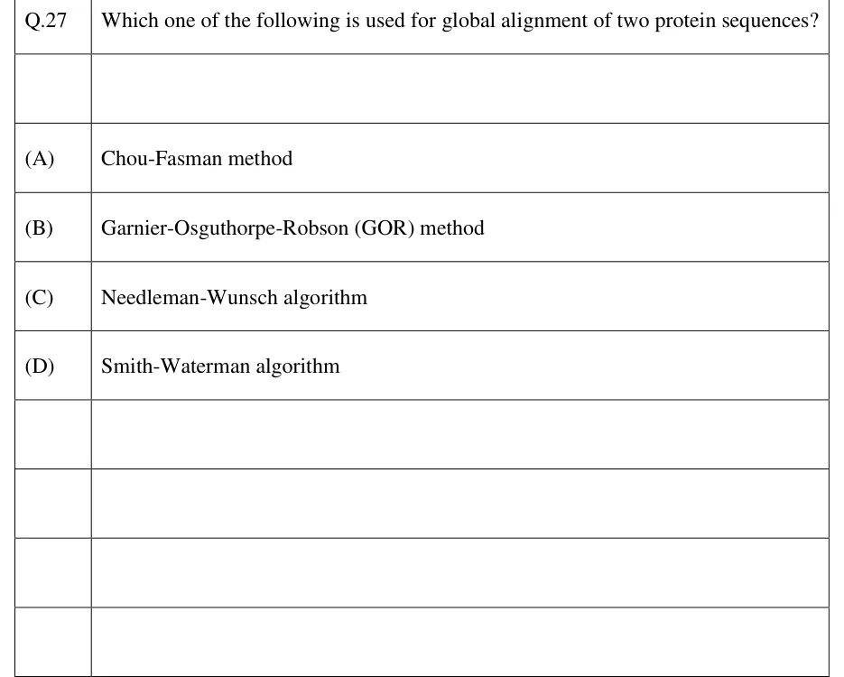
Global vs local alignment

Aspect

Global (Needleman–Wunsch)

Local (Smith–Waterman)

Aligns

The entire length of both sequences, end to end

The best-scoring sub-region only

Best used when

Sequences are of similar length and homologous over their whole length

Sequences share only a domain or motif, or differ greatly in length

Matrix initialisation

First row and column hold cumulative gap penalties

First row and column are 0

Traceback

Starts at the bottom-right cell and runs to the top-left

Starts at the highest-scoring cell anywhere; stops at the first cell with value 0

Negative cell values allowed?

Yes

No: any cell that would be negative is set to 0

GLOBAL ALIGNMENT RECURRENCE (NEEDLEMAN–WUNSCH)

F(i,j) = best score for aligning the first i residues of X with the first j residues of Y; = match/mismatch or matrix score; d = linear gap penalty, written as a positive number and subtracted. Initialisation: F(0,0) = 0, F(i,0) = −i·d, F(0,j) = −j·d. For sequences of lengths m and n this takes O(mn) time and memory.

LOCAL ALIGNMENT RECURRENCE (SMITH–WATERMAN)

The same as global alignment except for the 0 option and an initialisation of F(i,0) = F(0,j) = 0. The local alignment score is the largest F(i,j) anywhere in the matrix, and traceback stops at a cell with value 0.

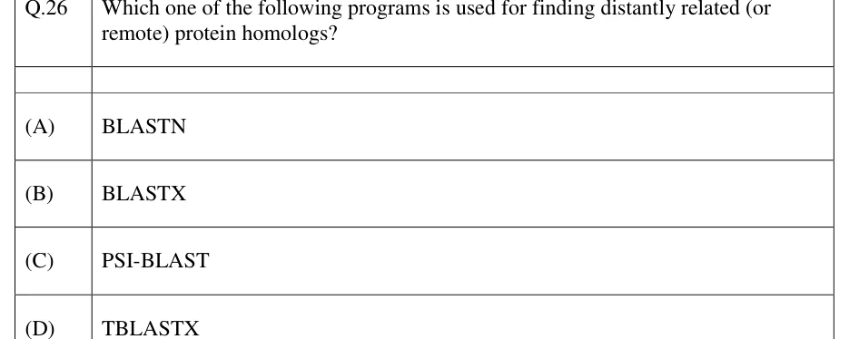
BLAST (Basic Local Alignment Search Tool) is a heuristic: it is fast, but it is not guaranteed to find the optimal alignment the way full dynamic programming does. (1) It breaks the query into short words (typically length 3 for proteins, 11 or more for nucleotides). For proteins it lists every 'neighbourhood' word that scores at least a threshold T against a query word under the substitution matrix. For nucleotides it uses exact word matches. (2) It scans the database for hits to these words. (3) It extends each hit in both directions and stops when the running score falls more than a set drop-off (X) below the best score reached. Gapped BLAST then performs a gapped extension on promising hits. (4) It reports the resulting HSPs (High-scoring Segment Pairs) whose significance passes the E-value cut-off. This trades some sensitivity for a very large gain in speed on whole databases.

BLAST programs

Program

Query

Database searched

blastn

Nucleotide

Nucleotide

blastp

Protein

Protein

blastx

Nucleotide, translated in all six reading frames

Protein

tblastn

Protein

Nucleotide, translated in all six reading frames

tblastx

Nucleotide, translated in six frames

Nucleotide, translated in six frames

BLAST E-VALUE (RAW SCORE)

E = the number of alignments with score ≥ S expected by chance alone in a search of this size; m = query length; n = total length of the database (in residues); S = the RAW alignment score; K and λ = statistical parameters of the scoring system. E rises in proportion to the search space (m·n) and falls exponentially as S rises. A smaller E-value means a more significant hit.

BIT SCORE, E-VALUE AND P-VALUE

The bit score S′ normalises the raw score so that scores from different scoring systems can be compared. Each extra bit halves E. P is the probability of at least one chance hit scoring ≥ S; when E is small (below about 0.01), P ≈ E.

Multiple sequence alignment (MSA) aligns three or more sequences at once to reveal conserved columns (motifs, active-site residues). It is the input for building profiles and HMMs and for phylogenetic trees. Exact MSA by dynamic programming grows roughly as for N sequences of length L, so practical tools use heuristic progressive alignment. They compute all pairwise distances, build a guide tree from them, align the closest pair first, and then add the next-closest sequence or profile. Its main weakness is that an error made in an early step, such as a misplaced gap, is carried forward and never revised ('once a gap, always a gap'). Iterative refinement methods re-align to reduce this.

WORKED EXAMPLE

Align X = ACGT and Y = AGT globally using match = +2, mismatch = −1 and a linear gap penalty of 2 per gap position (score −2). What is the optimal alignment score?

Solution
  1. Lengths are 4 and 3, so every global alignment needs one more gap in Y than in X. The fewest possible gaps is one gap in Y, giving 4 columns.

  2. Gap opposite A (ACGT / −AGT): −2 + (C,A) −1 + (G,G) +2 + (T,T) +2 = 1.

  3. Gap opposite C (ACGT / A−GT): (A,A) +2 − 2 + (G,G) +2 + (T,T) +2 = 4.

  4. Gap opposite G (ACGT / AC−T is not possible, since Y has no C; the alignment is ACGT / AG−T): (A,A) +2 + (C,G) −1 − 2 + (T,T) +2 = 1.

  5. Gap opposite T (ACGT / AGT−): +2 − 1 − 1 − 2 = −2.

  6. More gaps (one in X plus two in Y, 5 columns) allow at most 3 matches: 3(+2) − 3(2) = 0 or less, which cannot beat 4.

  7. The best is the gap opposite C.

Answer: Optimal global alignment score = 4, from ACGT / A−GT.

Phylogenetic trees

A phylogenetic tree shows inferred evolutionary relationships. Distance-based methods (UPGMA, Neighbor-Joining) first reduce the aligned sequences to a matrix of pairwise distances and then build the tree from that matrix. Character-based methods (Maximum Parsimony, Maximum Likelihood, Bayesian inference) work on the aligned characters column by column. They score each candidate tree against an explicit criterion and choose the best one.

UPGMA construction (Unweighted Pair Group Method with Arithmetic mean)

  1. Start with each sequence as its own cluster, and find the pair of clusters with the smallest distance.

  2. Join them at a node whose height is half that distance. UPGMA assumes a constant rate of change (a molecular clock), so both branches from the join are equally long.

  3. Recompute the distance from the merged cluster to every other cluster as the average of the original pairwise distances between their members, weighted by cluster size.

  4. Repeat until one cluster (the root) remains. The result is always a rooted, ultrametric tree: every leaf is the same distance from the root.

UPGMA DISTANCE UPDATE

The distance from the merged cluster (i,j) to cluster k is the average of the two distances, weighted by the numbers of sequences and in each cluster. This equals the plain average over all member pairs. Using the simple average without weights is a different method, WPGMA.

WORKED EXAMPLE

Build a UPGMA tree for four sequences with distances d(A,B) = 2, d(A,C) = 6, d(B,C) = 6, d(A,D) = 8, d(B,D) = 10, d(C,D) = 12. At what height is the root, and what are the leaf branch lengths?

Solution
  1. The smallest distance is d(A,B) = 2. Join A and B at height 2/2 = 1, so the branches to A and B are 1 each.

  2. Update: d(AB,C) = (1·6 + 1·6)/2 = 6; d(AB,D) = (1·8 + 1·10)/2 = 9; d(C,D) = 12 is unchanged.

  3. The smallest is d(AB,C) = 6. Join at height 3. The branch to C is 3, and the branch from node AB up to this node is 3 − 1 = 2.

  4. Update with size weights (AB has 2 members, C has 1): d(ABC,D) = (2·9 + 1·12)/3 = 30/3 = 10. Check: the average over the original pairs is (8 + 10 + 12)/3 = 10.

  5. Join ABC and D at height 10/2 = 5, which is the root. The branch to D is 5, and the branch from node ABC to the root is 5 − 3 = 2.

Answer: Root height = 5. Leaf branches: A = 1, B = 1, C = 3, D = 5. Internal branches: 2 (AB node to ABC node) and 2 (ABC node to root). Every leaf is at distance 5 from the root, so the tree is ultrametric.

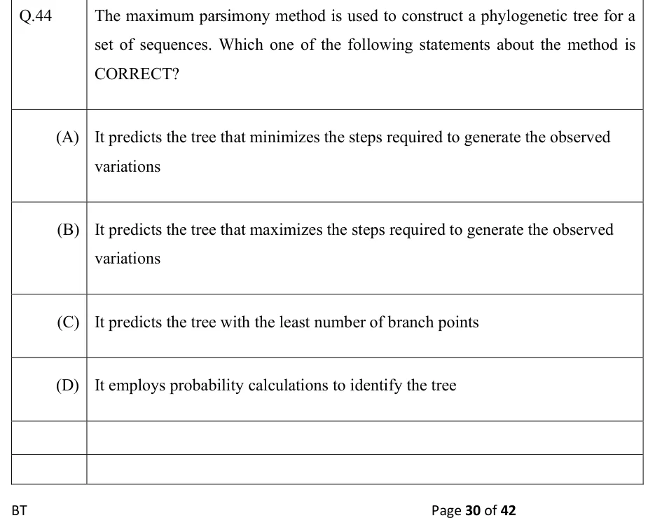
Maximum Parsimony: the guiding principle

  1. A site is parsimony-informative if at least two different character states each occur in at least two sequences.

  2. For each candidate topology, find the minimum number of character-state changes needed at each site to explain the data on that tree.

  3. Add these minima over all sites. Uninformative sites need the same number of changes on every topology, so only informative sites can tell topologies apart.

  4. Choose the topology with the smallest total, the most parsimonious tree. Several trees may tie.

Distance-based vs character-based methods

Method

Basis

Assumes molecular clock?

Produces

UPGMA

Pairwise distance matrix; clusters the closest pair

Yes

Rooted, ultrametric tree

Neighbor-Joining (NJ)

Pairwise distance matrix; greedy joining using the minimum-evolution criterion at each step

No

Unrooted tree with unequal branch lengths allowed (can be rooted with an outgroup)

Maximum Parsimony

Aligned characters; minimum total number of changes

No

Unrooted tree(s); several equally parsimonious trees are possible

Maximum Likelihood

Aligned characters plus an explicit substitution model; the tree with the highest probability of producing the data

No

Unrooted tree with branch lengths; computationally demanding

Bayesian inference

Aligned characters plus a substitution model and priors

No

Posterior probabilities of trees and clades

NUMBER OF POSSIBLE BIFURCATING TREES FOR N TAXA

Valid for n ≥ 3 (unrooted) and n ≥ 2 (rooted); !! is the double factorial (the product of odd numbers). Check: n = 4 gives 3 unrooted and 15 rooted trees; n = 5 gives 15 unrooted and 105 rooted trees. The number of rooted trees for n taxa equals the number of unrooted trees for n + 1 taxa.

Tree terminology

  1. An unrooted binary tree of n leaves has n − 2 internal nodes and 2n − 3 branches. A rooted binary tree has n − 1 internal nodes and 2n − 2 branches.

  2. Rooting with an outgroup: add a taxon known to lie outside the group being studied. The root is placed on the branch where the outgroup joins.

  3. Phylogram: branch lengths are drawn to scale and show the amount of change. Cladogram: it shows branching order only, and branch lengths mean nothing.

  4. Bootstrap support: resample alignment columns with replacement to create many pseudo-alignments, build a tree from each, and report the percentage of those trees that contain a given clade.

EXAM TIP

Rotating the branches at any internal node does not change the relationships a tree shows, so the top-to-bottom order of leaves on the page means nothing. Relatedness is read from the most recent common ancestor. A tree is unrooted unless a root or outgroup is shown, and an unrooted tree cannot tell you the direction of evolution.

Gene prediction, functional annotation and structure prediction

Approaches to gene prediction

  1. Open reading frame (ORF): a stretch that begins at a start codon (usually ATG) and runs in frame to a stop codon (TAA, TAG or TGA). A DNA sequence has six reading frames, three on each strand.

  2. Ab initio (intrinsic): looks for statistical signals of coding regions in the sequence alone, such as long ORFs, codon-usage bias, start and stop codons, splice sites and promoter or ribosome-binding motifs. Often implemented with hidden Markov models. It is simpler in prokaryotes (continuous ORFs, few introns) than in eukaryotes, where exon–intron structure must be predicted.

  3. Homology-based (extrinsic): aligns the sequence against known proteins, cDNAs, ESTs or RNA-seq transcripts. A significant match is supporting evidence for a gene and for its exon structure.

  4. Comparative genomics: aligns genomes of related species. Functional regions are under selection and stay conserved while non-functional DNA drifts, so conservation flags likely genes and regulatory elements.

Functional annotation assigns a probable biological role to a predicted gene or protein. The main routes are (i) similarity search against annotated sequence databases; (ii) matching domain, motif and family signatures (PROSITE, Pfam, InterPro), which can suggest a function even without similarity over the full length; (iii) assigning Gene Ontology (GO) terms in its three aspects, molecular function, biological process and cellular component; and (iv) mapping the gene product onto pathway databases such as KEGG to place it in a metabolic or signalling context. Annotation transferred by similarity is a prediction, not an experimental result.

Secondary-structure prediction assigns each residue to one of three states: helix (H), strand (E) or coil (C). Early methods (Chou–Fasman, GOR) used the statistical preference of each amino acid, or of a window of residues, for each state. Later methods, often neural networks, use evolutionary information from multiple alignments and are more accurate. Tertiary (3-D) structure prediction uses homology (comparative) modelling, threading (fold recognition) or ab initio/de novo modelling. Deep-learning methods trained on known structures and on co-evolution signals in multiple alignments now predict many protein structures with high accuracy. Any model is checked for stereochemical quality, for example with a Ramachandran plot of backbone φ/ψ angles.

3-D structure prediction strategies

Strategy

Requires

Best when

Homology (comparative) modelling

A solved structure of a homolog (the template) and a reliable sequence alignment to it

A clear homolog exists. As a rough rule of thumb, it is dependable when identity is about 30% or more over the aligned region

Threading / fold recognition

A library of known folds; no detectable sequence homolog needed

Sequence identity to every solved structure is too low for comparative modelling, but the fold is probably already known

Ab initio / de novo

Only the sequence plus an energy or scoring function and a conformational search

No usable template or fold match exists; most practical for small proteins

Genomics, proteomics, metabolomics, metagenomics and systems biology

The -omics layers

Field

Studies

Typical methods

Typical output

Genomics

The complete DNA sequence and genes of an organism

Genome sequencing, assembly, gene prediction

Assembled genome, gene models, annotation

Transcriptomics

The complete set of RNA transcripts in a cell or tissue under given conditions

RNA-seq, DNA microarrays

Which genes are expressed and at what level

Proteomics

The complete set of proteins expressed by a cell or tissue at a given time

2-D gel electrophoresis (isoelectric focusing, then SDS-PAGE); mass spectrometry (MALDI-TOF, ESI-MS/MS); peptide mass fingerprinting

Protein identities, abundances, post-translational modifications

Metabolomics

The complete set of small-molecule metabolites present

NMR, GC-MS, LC-MS

Metabolite profiles and concentrations

Metagenomics

Genetic material recovered directly from an environmental sample (a mixed community), without culturing individual organisms

Amplicon (e.g. 16S rRNA) or shotgun sequencing of environmental DNA

Community composition and, from shotgun data, the community's gene content

A typical metagenomics workflow

  1. Extract DNA directly from the environmental sample (soil, gut, water), with no culturing step.

  2. Amplicon route: PCR-amplify and sequence a marker gene (16S rRNA for bacteria and archaea), then classify the reads against reference databases. This gives a taxonomic profile ('who is there'), not the community's gene content.

  3. Shotgun route: sequence all the DNA, assemble reads into contigs, and group contigs into bins that approximate individual genomes, or classify reads directly.

  4. On shotgun assemblies, predict genes, annotate them functionally and combine the results across the community to infer its collective metabolic capability ('what they can do').

Systems biology combines genome-scale data (genomic, transcriptomic, proteomic, metabolomic) into quantitative models of how whole cells behave, instead of studying one gene or pathway at a time. Metabolic engineering uses this understanding to redesign an organism's metabolic network on purpose, for example to raise the yield of a target compound by deleting competing pathways or over-expressing bottleneck enzymes. It is often guided by a genome-scale metabolic model.

FLUX BALANCE ANALYSIS (FBA)

S = stoichiometric matrix (rows = metabolites, columns = reactions); v = vector of reaction fluxes. At steady state the net rate of change of every internal metabolite is zero, giving one linear equation per metabolite. The bounds encode irreversibility and uptake limits. c selects the objective (e.g. biomass or product flux). The problem is solved by linear programming, not by simulating dynamics. Before the bounds are applied, the steady-state solutions form a space of dimension (number of reactions) − rank(S).

EXAM TIP

Knowledge discovery (data mining) in biochemical databases, such as clustering genes by expression pattern or mining co-occurring pathway annotations, works on top of the -omics data described above. It is a data-analysis layer, not a separate experimental technique.

PREVIOUS-YEAR QUESTIONS

11 questions from the BT papers

Try each question first, then open the answer. One shows the official answer only. We placed each question under a topic ourselves; the exam paper does not label topics.

See these papers in full: GATE BT 2026 · GATE BT 2025 · GATE BT 2023 · GATE BT 2022 · GATE BT 2020 · GATE BT 2019

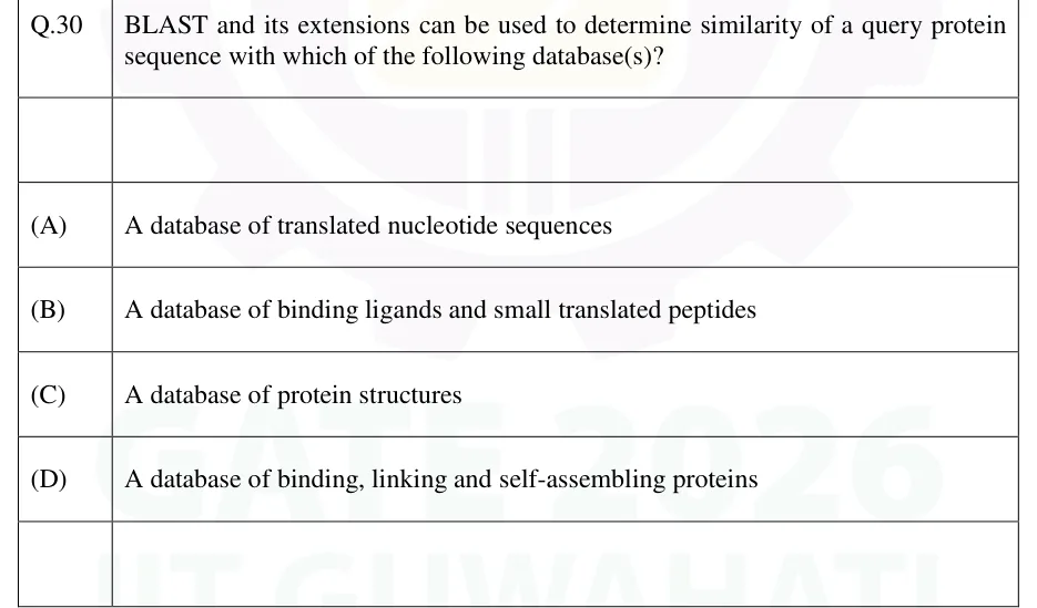
GATE 2026 BT Q.30

GATE 2026 · BTQ.30 · 1 mark · MSQ

BLAST and its extensions can be used to determine similarity of a query protein sequence with which of the following database(s)?

  1. (A)

    A database of translated nucleotide sequences

  2. (B)

    A database of binding ligands and small translated peptides

  3. (C)

    A database of protein structures

  4. (D)

    A database of binding, linking and self-assembling proteins

Official answer
See the question in the paper
GATE 2026 BT Q.30: official answer

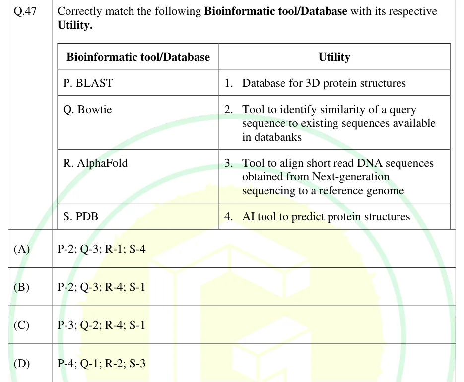
GATE 2025 BT Q.47

GATE 2025 · BTQ.47 · 2 marks · MCQ

Correctly match the following Bioinformatic tool/Database with its respective Utility.

Bioinformatic tool/Database:
P. BLAST
Q. Bowtie
R. AlphaFold
S. PDB

Utility:
1. Database for 3D protein structures
2. Tool to identify similarity of a query sequence to existing sequences available in databanks
3. Tool to align short read DNA sequences obtained from Next-generation sequencing to a reference genome
4. AI tool to predict protein structures

  1. (A)

    P-2; Q-3; R-1; S-4

  2. (B)

    P-2; Q-3; R-4; S-1

  3. (C)

    P-3; Q-2; R-4; S-1

  4. (D)

    P-4; Q-1; R-2; S-3

Answer and solution
See the question in the paper
GATE 2025 BT Q.47: answer and solution

GATE 2022 BT Q.44

GATE 2022 · BTQ.44 · 2 marks · MCQ

The maximum parsimony method is used to construct a phylogenetic tree for a set of sequences. Which one of the following statements about the method is CORRECT?

  1. (A)

    It predicts the tree that minimizes the steps required to generate the observed variations

  2. (B)

    It predicts the tree that maximizes the steps required to generate the observed variations

  3. (C)

    It predicts the tree with the least number of branch points

  4. (D)

    It employs probability calculations to identify the tree

Answer and solution
See the question in the paper
GATE 2022 BT Q.44: answer and solution

GATE 2020 BT Q.54

GATE 2020 · BTQ.54 · 2 marks · NAT

Q.No. 54 An algorithm was designed to find globins in protein sequence databases. A database which has 78 globin sequences was searched using this algorithm. The algorithm retrieved 72 sequences of which only 65 were globins. The sensitivity of this algorithm is ________ % (round off to 2 decimal places).

Answer and solution
See the question in the paper
GATE 2020 BT Q.54: answer and solution

GATE 2019 BT Q.29

GATE 2019 · BTQ.29 · 2 marks · MCQ

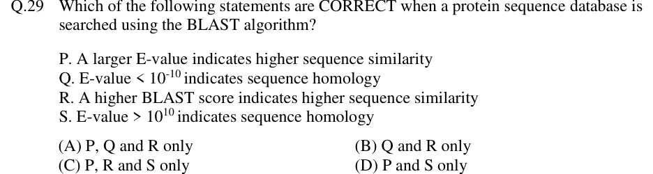
Which of the following statements are CORRECT when a protein sequence database is searched using the BLAST algorithm?

P. A larger E-value indicates higher sequence similarity
Q. E-value < 10^-10 indicates sequence homology
R. A higher BLAST score indicates higher sequence similarity
S. E-value > 10^10 indicates sequence homology

  1. (A)

    P, Q and R only

  2. (B)

    Q and R only

  3. (C)

    P, R and S only

  4. (D)

    P and S only

Answer and solution
See the question in the paper
GATE 2019 BT Q.29: answer and solution

PRACTICE

7 questions to test yourself

PRACTICE 11 mark · MCQ

Which of the following correctly matches a bioinformatics resource with its primary content?

  1. (A)

    PDB — curated pathway maps

  2. (B)

    Pfam — 3-D atomic coordinates of proteins

  3. (C)

    UniProtKB/Swiss-Prot — manually reviewed protein sequences and annotation

  4. (D)

    KEGG — raw unassembled sequencing reads

Answer and solution

Answer: (C)

  1. PDB stores experimentally determined 3-D structures, not pathways, so A is wrong.

  2. Pfam stores protein domain families (profile HMMs built from alignments), not coordinates, so B is wrong.

  3. KEGG stores pathway maps linked to genes and compounds, not raw reads, so D is wrong.

  4. Swiss-Prot is the manually reviewed section of UniProtKB, so C is correct.

PRACTICE 21 mark · NAT

A genome-scale metabolic model has a stoichiometric matrix S of size 25 metabolites × 40 reactions, and S has full row rank. How many independent linear constraint equations does the steady-state condition S·v = 0 impose on the flux vector v?

Answer and solution

Answer:

  1. The steady-state condition S·v = 0 gives one equation per row of S, that is, one per metabolite: 25 equations.

  2. S has full row rank, so all 25 rows are linearly independent and none is redundant.

  3. So there are 25 independent constraint equations. (Consequently the steady-state flux space, before bounds, has dimension 40 − 25 = 15.)

PRACTICE 31 mark · NAT

How many distinct unrooted, fully bifurcating tree topologies are possible for 5 taxa?

Answer and solution

Answer:

  1. Use N_unrooted(n) = (2n − 5)!! = (2n − 5)! / [2^(n−3) (n − 3)!].

  2. For n = 5: (2·5 − 5)!! = 5!! = 5 × 3 × 1 = 15.

  3. Check with the factorial form: 5! / (2^2 × 2!) = 120 / 8 = 15.

PRACTICE 41 mark · MCQ

A researcher has a protein sequence and wants to find genomic regions in an unannotated nucleotide database that could encode similar proteins. Which BLAST program is appropriate?

  1. (A)

    blastx

  2. (B)

    tblastn

  3. (C)

    tblastx

  4. (D)

    blastn

Answer and solution

Answer: (B)

  1. The query is a protein and the database is nucleotide.

  2. tblastn compares a protein query against a nucleotide database translated in all six reading frames, so B is correct.

  3. blastx is the reverse (a translated nucleotide query against a protein database); tblastx translates both query and database, and needs a nucleotide query; blastn compares nucleotide against nucleotide.

PRACTICE 52 marks · NAT

Align X = ACGT and Y = CGTA by global (Needleman–Wunsch) alignment with match = +2, mismatch = −1 and a linear gap penalty of 2 per gap position (score −2). What is the optimal alignment score?

Answer and solution

Answer:

  1. Without gaps (4 columns) every column mismatches: A/C, C/G, G/T, T/A give 4(−1) = −4.

  2. Both sequences share the subsequence CGT, offset by one position. With one gap in each sequence, ACGT− / −CGTA, the columns score −2 + 2 + 2 + 2 − 2 = 2.

  3. Because the lengths are equal, any gapped alignment has equal numbers of gaps in X and Y, so at least 2 gap positions. No alignment can have more than 3 matches, because CGT is the longest common subsequence. So every gapped alignment scores at most 3(2) − 2(2) = 2.

  4. Full dynamic programming confirms it: with F(i,0) = −2i and F(0,j) = −2j, the matrix gives F(4,4) = 2, reached via F(3,2) = 2 and F(4,3) = 4 on the CGT diagonal.

PRACTICE 62 marks · MSQ

Which of the following statements about UPGMA and Neighbor-Joining (NJ) are TRUE?

  1. (A)

    UPGMA assumes a constant rate of evolution (molecular clock) across all lineages

  2. (B)

    Neighbor-Joining does not require a constant rate of evolution across lineages

  3. (C)

    UPGMA always produces an unrooted tree

  4. (D)

    Both UPGMA and Neighbor-Joining are distance-based (not character-based) methods

Answer and solution

Answer: (A), (B), (D)

  1. UPGMA places each join at half the distance, giving equal branch lengths, which is valid only under a molecular clock. A is true.

  2. NJ corrects for unequal rates when choosing which pair to join and allows unequal branch lengths. B is true.

  3. UPGMA produces a rooted, ultrametric tree (the root is the last merge). C is false.

  4. Both methods build the tree from a pairwise distance matrix, not from aligned characters. D is true.

PRACTICE 71 mark · MCQ

In the BLAST E-value formula E = K m n e^(−λS) (m = query length, n = database size, S = raw alignment score), if the database size n is increased while m, S, K and λ are held fixed, the E-value:

  1. (A)

    Decreases

  2. (B)

    Increases

  3. (C)

    Stays exactly the same

  4. (D)

    Becomes exactly zero

Answer and solution

Answer: (B)

  1. E is directly proportional to n in E = K m n e^(−λS).

  2. With every other quantity fixed, increasing n increases E in proportion.

  3. This matches the idea that a larger database gives more chances for a given score to arise by chance.

OFFICIAL GATE 2027 SYLLABUS WORDING

Copied from the GATE 2027 syllabus; see all 2027 syllabi.

GATE BT

Bioinformatics resources and search tools; Sequence and structure databases; Sequence analysis - sequence file formats, scoring matrices, alignment, phylogeny; Genomics, proteomics, metabolomics; Gene prediction; Functional annotation; Secondary structure and 3D structure prediction; Knowledge discovery in biochemical databases; Metagenomics; Metabolic engineering and systems biology

Preparing in Kolkata? IAE Academy's course for GATE BT.