GATE BT

Measurement, dynamics and process control

Process control keeps a bioreactor's temperature, pH, dissolved oxygen, pressure, level and flows at their set points. A sensor measures each variable, a controller compares it with the set point, and a valve or pump acts on the error. The calculations in this topic are the step, ramp and sinusoidal responses of first- and second-order systems (time constant, damping ratio, overshoot, decay ratio), closed-loop transfer functions, the offset left by proportional control, Routh and Bode stability and the ultimate gain, and Ziegler–Nichols or Cohen–Coon tuning settings. Conventions used throughout: deviation variables, controller error $e = y_{s p} - y_{m}$ , time constants in the time unit of the problem, and natural logarithms unless $lo g_{10}$ is written.

9 previous-year questions · 9 solved · 6 practice questions

Measurement devices and control valves

A control loop can be no better than its measurement. In a bioreactor the routinely measured variables are temperature, pressure, liquid and gas flow, level (and foam), pH and dissolved oxygen (DO). Off-gas $O_{2}$ and $C O_{2}$ are also analysed, to calculate the oxygen uptake rate, the carbon dioxide evolution rate and the respiratory quotient. A probe that sits inside the sterile boundary must survive steam sterilisation in place, and every sensor adds its own small lag to the loop.

Variable	Common devices	Principle and key point
Temperature	RTD (Pt-100), thermocouple, thermistor	RTD resistance rises almost linearly with temperature (Pt-100 = 100 Ω at 0 °C). A thermocouple gives an emf from the Seebeck effect that depends on the temperature difference between its measuring junction and a reference (cold) junction, so the reference temperature must be known or compensated. An NTC thermistor's resistance falls steeply and non-linearly with temperature. A probe in a thermowell adds a first-order lag.
Pressure	Diaphragm with strain gauge or piezoresistive element; Bourdon gauge	Head-space pressure sets the $O_{2}$ partial pressure, and so the saturation DO (Henry's law). It also feeds the safety interlocks.
Liquid flow	Orifice or venturi (differential pressure), rotameter, electromagnetic, Coriolis	Differential-pressure meters give $Q \propto Δ P$ . An electromagnetic meter needs a conducting liquid. A Coriolis meter reads mass flow directly.
Gas flow	Rotameter, thermal mass-flow meter	A thermal meter, calibrated for the gas composition, reads mass (standard) flow, which does not depend on gas temperature or pressure.
Level and foam	Differential-pressure cell, load cells, capacitance or conductance probes	A conductance foam probe switches antifoam addition on and off (two-position control).
pH	Combination glass electrode (glass membrane plus Ag/AgCl reference)	The potential follows the Nernst equation, with a slope of 59.16 mV per pH unit at 25 °C. The slope is proportional to absolute temperature, so the meter is temperature-compensated and calibrated with two buffers.
Dissolved oxygen	Polarographic (Clark) electrode, galvanic electrode, optical (luminescence) sensor	In a Clark electrode a platinum or gold cathode is polarised by an applied voltage against an Ag/AgCl anode; a galvanic electrode generates its own polarising voltage. The current is proportional to the $O_{2}$ flux through the membrane, i.e. to the $O_{2}$ partial pressure, and the reading is usually given in % air saturation. The membrane adds a lag, which matters when $k_{L} a$ is measured by the dynamic method. An optical sensor consumes no oxygen.
Off-gas	Paramagnetic $O_{2}$ analyser, infrared $C O_{2}$ analyser, mass spectrometer	Inlet and outlet compositions give the OUR, the CER and $R Q = CER / OUR$ .

RESISTANCE THERMOMETER (RTD)

R_{T} = R_{0} (1 + α T), α \approx 0.00385^{\circ} C^{- 1} (platinum)

$T$ in °C and $R_{0}$ the resistance at 0 °C. A linear approximation, good over moderate ranges.

PH ELECTRODE (NERNST)

E = E^{0} - \frac{2.303 R T}{F} pH, \frac{2.303 R T}{F} = 59.16 mV per pH at 298 K

$E^{0}$ is a constant of the electrode pair, fixed by calibration with buffers. $R = 8.314$ J mol $^{- 1}$ K $^{- 1}$ , $F = 96485$ C mol $^{- 1}$ , $T$ in K. The slope is proportional to absolute temperature.

ORIFICE OR VENTURI FLOW METER

Q = C_{d} A_{0} \frac{2 Δ P}{ρ ( 1 - β ^{4} )}, β = \frac{d _{0}}{D}

SI units: $Q$ in m $^{3}$ s $^{- 1}$ , $Δ P$ in Pa, $ρ$ (fluid density) in kg m $^{- 3}$ . $A_{0}$ and $d_{0}$ are the orifice (or venturi throat) area and diameter, $D$ is the pipe diameter and $C_{d}$ the discharge coefficient. Because $Q \propto Δ P$ , a 10 : 1 flow range needs a 100 : 1 pressure-drop range.

The control valve is the usual final control element. A pneumatic actuator (3–15 psig, i.e. about 20–100 kPa gauge, or 4–20 mA through an I/P converter) moves the stem. Air-to-open means fail-closed and air-to-close means fail-open, and which one to use is decided by what is safe when air or power is lost. The valve's inherent characteristic relates the fraction of maximum flow $f$ to the fractional stem lift $x$ ( $0 \leq x \leq 1$ ) at constant pressure drop across the valve. The rangeability $R$ is the ratio of the maximum to the minimum controllable flow; values of 20 to 50 are common.

VALVE FLOW EQUATION

q = C_{v} f (x) \frac{Δ P _{v}}{s.g.}

US customary units: $q$ in US gal/min, $Δ P_{v}$ (pressure drop across the valve) in psi. $C_{v}$ is the valve coefficient (the flow of water in US gal/min through the fully open valve at a 1 psi drop), s.g. the specific gravity of the liquid, and $f (x)$ the inherent characteristic.

INHERENT VALVE CHARACTERISTICS

Linear: Equal percentage: Quick opening: f = x f = R^{x - 1}, \frac{1}{f} \frac{df}{d x} = ln R f = x

At constant valve pressure drop; the quick-opening form is one common idealisation. For an equal-percentage valve, equal increments of stem travel give equal fractional changes in flow. The ideal equal-percentage curve gives $f = 1/ R$ at $x = 0$ , the minimum controllable flow; a real valve departs from the curve near closure and shuts off.

Characteristic	Slope $df / d x$	When it is chosen
Linear	Constant (= 1)	When the valve takes most of the system pressure drop, so that $Δ P_{v}$ stays nearly constant
Equal percentage	$f ln R$ , grows with flow	When line losses are large, so $Δ P_{v}$ falls as flow rises (the installed characteristic then becomes close to linear), or when a wide range of flow is needed
Quick opening	$\frac{1}{2 x}$ , large near closed	On/off service

EXAM TIP

Fail-safe choice. Cooling water to the jacket of an exothermic fermentation should fail open (air-to-close), so that losing instrument air cannot let the broth overheat. A steam, acid, base or substrate feed valve normally fails closed (air-to-open). With the valve gain defined as change in flow per unit change in controller output, an air-to-close valve has a negative gain ( $K_{v} < 0$ ), so the controller action must be the opposite of the one used with an air-to-open valve to keep the loop in negative feedback (see the section on controllers).

EXAM TIP

Transmitter gain = span of the output signal ÷ span of the measured variable. A transmitter giving 4–20 mA over 20–120 °C has a range of 20–120 °C, a zero of 20 °C and a span of 100 °C, so $K_{m} = 16/100 = 0.16$ mA/°C. The 4 mA live zero does not enter the gain.

Deviation variables, transfer functions and block diagrams

Control calculations use deviation variables, $y^{'} (t) = y (t) - \overset{y}{ˉ}$ , where $\overset{y}{ˉ}$ is the initial steady state. Every initial condition is then zero, and the transfer function $G (s) = Y^{'} (s) / U^{'} (s)$ is the Laplace transform of the linear (or linearised) model. For a self-regulating process the steady-state gain is $K = G (0)$ , the final change in output per unit change in input. Poles are the roots of the denominator: all of them in the left half of the $s$ -plane means the system is stable.

LAPLACE TRANSFORMS USED IN PROCESS DYNAMICS

L {M u (t)} L {e^{- a t}} L {\frac{d y}{d t}} L {f (t - θ) u (t - θ)} = \frac{M}{s}, L {a t} = \frac{a}{s ^{2}}, L {A δ (t)} = A = \frac{1}{s + a}, L {sin ω t} = \frac{ω}{s ^{2} + ω ^{2}} = s Y (s) - y (0), L {\int_{0}^{t} y d t} = \frac{Y ( s )}{s} = e^{- θ s} F (s)

One-sided transforms of functions defined for $t \geq 0$ . $u (t)$ is the unit step and $δ (t)$ the unit impulse. $e^{- θ s}$ is a pure dead time (transport lag) of $θ$ .

FINAL AND INITIAL VALUE THEOREMS

t \to \infty lim y (t) = s \to 0 lim s Y (s), t \to 0^{+} lim y (t) = s \to \infty lim s Y (s)

The final value theorem holds only if $y (t)$ settles, i.e. every pole of $s Y (s)$ has a negative real part. Applied to an unstable or sustained-oscillation response, it returns a meaningless number.

PADÉ APPROXIMATION OF DEAD TIME

e^{- θ s} \approx \frac{1 - θ s /2}{1 + θ s /2}

First-order approximation, used to bring dead time into a polynomial characteristic equation (for example before a Routh test).

BLOCK-DIAGRAM ALGEBRA

Series: G_{1} G_{2}, Parallel: G_{1} \pm G_{2}, Negative feedback: \frac{G}{1 + G H}, Positive feedback: \frac{G}{1 - G H}

$G$ is the forward-path and $H$ the feedback-path transfer function.

CLOSED-LOOP RESPONSE OF A FEEDBACK LOOP

Y (s) = \frac{G _{c} G _{v} G _{p}}{1 + G _{c} G _{v} G _{p} G _{m}} Y_{s p} (s) + \frac{G _{d}}{1 + G _{c} G _{v} G _{p} G _{m}} D (s)

$G_{c}$ = controller, $G_{v}$ = valve, $G_{p}$ = process, $G_{m}$ = measuring element, $G_{d}$ = disturbance path. $G_{O L} = G_{c} G_{v} G_{p} G_{m}$ is the open-loop transfer function. The equation assumes the set point and the measurement are in the same units. If the set point is entered in process units while $K_{m} \neq = 1$ , the servo numerator carries an extra factor $K_{m}$ .

Reading a closed-loop problem

Servo problem: the set point changes and $D = 0$ . Regulator (load) problem: the disturbance changes and $Y_{s p}$ is held.
The characteristic equation $1 + G_{O L} (s) = 0$ is the same for both, so stability does not depend on where the input enters.
Offset $= y_{s p} (\infty) - y (\infty)$ , found from the final value theorem on the closed-loop expression (only for a stable loop).
Convert absolute values to deviations first (a set point moved from 37 °C to 38 °C is a step of +1 °C), then add the answer back to the old steady state.

First-order systems

A first-order system has a single capacity (for mass, energy or volume), and its model is $τ \frac{d y}{d t} + y = K u$ in deviation variables. The time constant $τ$ is the ratio of capacity to resistance (or of hold-up to throughput), and the gain $K$ has the units of output per unit input. First-order models describe a thermometer or DO probe, a stirred tank's temperature or concentration, and a tank level with a resistive outflow.

FIRST-ORDER TRANSFER FUNCTION

G (s) = \frac{Y ( s )}{U ( s )} = \frac{K}{τ s + 1}

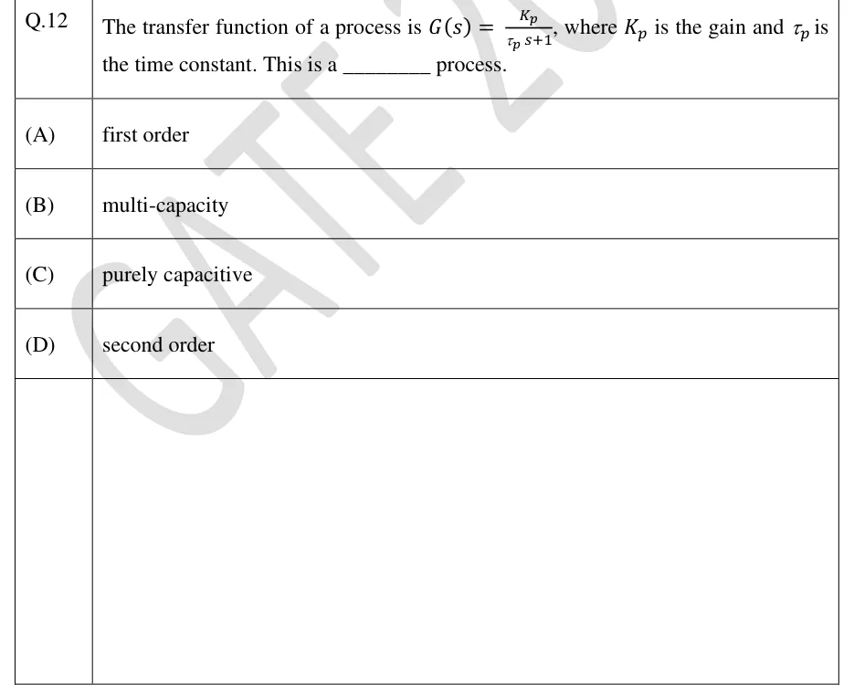
$K$ = steady-state gain; $τ$ = time constant (in time units). The pole is at $s = - 1/ τ$ .

System	Model (deviation form)	Gain $K$	Time constant $τ$
Thermometer or thermowell (surroundings at $T_{s}$ )	$m C_{p} \frac{d T}{d t} = h A (T_{s} - T)$	1	$\frac{m C _{p}}{h A}$
Tank, outflow through a linear resistance $q_{o} = h / R$	$A \frac{d h}{d t} = q_{i} - \frac{h}{R}$	$R$ (for $h$ vs $q_{i}$ )	$A R$
Well-mixed vessel, constant volume $V$ and flow $F$	$V \frac{d C}{d t} = F (C_{i} - C)$	1	$\frac{V}{F}$
Well-mixed vessel with first-order reaction (rate constant $k$ )	$V \frac{d C}{d t} = F (C_{i} - C) - k V C$	$\frac{F}{F + k V}$	$\frac{V}{F + k V}$

LINEARISED OUTFLOW RESISTANCE

q_{o} = C h \Rightarrow R = (\frac{d q _{o}}{d h})_{\overset{ˉ}{h}}^{- 1} = \frac{2 h ˉ}{C} = \frac{2 h ˉ}{q ˉ _{o}}

Taylor linearisation about the steady state $\overset{ˉ}{h}$ . Valid only for small deviations. Then $τ = A R$ .

STEP RESPONSE (INPUT STEP OF SIZE M)

y (t) = K M (1 - e^{- t / τ}), t_{f} = τ ln \frac{1}{1 - f}

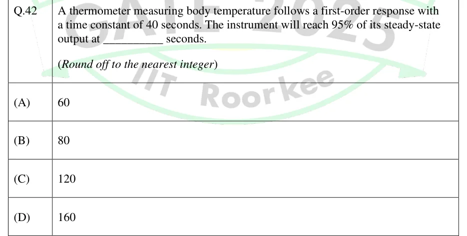
$y$ reaches 63.2% of its final change $K M$ at $t = τ$ , 86.5% at $2 τ$ , 95.0% at $3 τ$ , 98.2% at $4 τ$ and 99.3% at $5 τ$ . The initial slope is $K M / τ$ , so the tangent at $t = 0$ meets the final value at $t = τ$ . $t_{f}$ is the time to reach a fraction $f$ of the final change (natural log).

IMPULSE RESPONSE (IMPULSE OF AREA A)

y (t) = \frac{K A}{τ} e^{- t / τ}

The output jumps to $K A / τ$ at $t = 0^{+}$ and then decays back to the old steady state.

RAMP RESPONSE (INPUT U = A T)

y (t) = K a (t - τ + τ e^{- t / τ}) \to K a (t - τ) for t ≫ τ

After the transient dies out, the output follows the ramp but lags it by a time $τ$ . For a sensor ( $K = 1$ ) the reading trails the true value by $a τ$ .

SINUSOIDAL (FREQUENCY) RESPONSE

u = A sin ω t \Rightarrow y = \hat{A} sin (ω t + ϕ), \frac{A ^}{A} = \frac{K}{1 + ω ^{2} τ ^{2}}, ϕ = - tan^{- 1} (ω τ)

Ultimate periodic response, after the transient has decayed. $ω$ in rad per unit time. This amplitude ratio includes the gain $K$ ; dividing by $K$ gives the normalised amplitude ratio. The lag is 45° at $ω τ = 1$ and approaches, but never reaches, 90°.

FIRST ORDER PLUS DEAD TIME (FOPDT)

G (s) = \frac{K e ^{- θ s}}{τ s + 1}

The standard model fitted to a process reaction curve. Dead time adds a phase lag of $ω θ$ rad (a phase angle of $- ω θ$ , with no upper limit) and leaves the amplitude ratio unchanged.

INTEGRATING (PURE CAPACITIVE) PROCESS

G (s) = \frac{H ( s )}{Q _{i} ( s )} = \frac{1}{A s}

A tank whose outflow is fixed by a pump: a step in inflow gives a ramp in level that never settles. The process is not self-regulating, and the final value theorem does not apply to it ( $s Y (s)$ has a pole at $s = 0$ ).

TWO TANKS IN SERIES

Non-interacting: Interacting: \frac{H _{2} ( s )}{Q _{i} ( s )} = \frac{R _{2}}{( τ _{1} s + 1 ) ( τ _{2} s + 1 )} \frac{H _{2} ( s )}{Q _{i} ( s )} = \frac{R _{2}}{τ _{1} τ _{2} s ^{2} + ( τ _{1} + τ _{2} + A _{1} R _{2} ) s + 1}

Linear outflow resistances, $τ_{1} = A_{1} R_{1}$ , $τ_{2} = A_{2} R_{2}$ . In the non-interacting case tank 1 drains freely into tank 2. In the interacting case the flow between the tanks is $(h_{1} - h_{2}) / R_{1}$ . Both are overdamped, and interaction adds the term $A_{1} R_{2}$ , which makes the response more sluggish. The steady-state gain is $R_{2}$ in both.

WORKED EXAMPLE

A temperature sensor in a thermowell behaves as a first-order element with unit gain and $τ = 1.2$ min. The broth is at a steady 30 °C when heating for in-situ sterilisation starts, and the true temperature then rises at a constant 0.5 °C/min. Find (a) the sensor reading, and the error, 3 min after the ramp starts, and (b) the error once the transient has died out.

Solution

In deviation form the input is $T^{'} (t) = a t$ with $a = 0.5$ °C/min, so $T^{'} (s) = a / s^{2}$ .
Measured deviation: $Y (s) = \frac{a}{s ^{2} ( τ s + 1 )}$ , which inverts to $y^{'} (t) = a (t - τ + τ e^{- t / τ})$ .
At $t = 3$ min: $y^{'} = 0.5 (3 - 1.2 + 1.2 e^{- 2.5}) = 0.5 (1.8 + 1.2 \times 0.0821) = 0.949$ °C, so the reading is 30.95 °C.
True temperature at 3 min: $30 + 0.5 \times 3 = 31.50$ °C. Error $= 31.50 - 30.95 = 0.55$ °C.
For $t ≫ τ$ : $y^{'} \to a (t - τ)$ . The reading runs $τ = 1.2$ min behind the true temperature, an error of $a τ = 0.5 \times 1.2 = 0.60$ °C.

Answer: (a) Reading 30.95 °C, error about 0.55 °C. (b) A steady lag error of 0.60 °C (the reading is 1.2 min behind).

EXAM TIP

The '63.2% at one time constant' rule holds for a step input only. For a ramp input the lasting effect is a lag error of $K a τ$ (a lag of $τ$ in time). For a sinusoid, the attenuation and phase lag come from the amplitude-ratio formula. Before using any of these, check which input the question gives.

Second-order systems

Second-order behaviour comes from two first-order lags in series, from a system with inertia (for example a valve actuator or a manometer), and from feedback: a first-order process under PI control, or a process with one lag under P control through a valve or sensor that has another lag. (A first-order process under P control alone with pure-gain valve and sensor stays first order.) For the standard form below, which has no numerator zero, only complex poles ( $ζ < 1$ ) give overshoot. Two first-order lags in series always have $ζ \geq 1$ .

STANDARD SECOND-ORDER TRANSFER FUNCTION

G (s) = \frac{K}{τ ^{2} s ^{2} + 2 ζ τ s + 1} = \frac{K ω _{n}^{2}}{s ^{2} + 2 ζ ω _{n} s + ω _{n}^{2}}, ω_{n} = \frac{1}{τ}

$K$ = gain, $ζ$ = damping ratio, $ω_{n}$ = natural frequency (rad per unit time), and $τ = 1/ ω_{n}$ , which is conventionally called the natural period of oscillation (the undamped oscillation actually repeats every $2 π τ$ ). Put the constant term of the denominator equal to 1 before reading off $K$ , $τ$ and $ζ$ .

Damping ratio	Poles	Step response
$ζ > 1$	Two real, distinct, negative	Overdamped: sluggish, no overshoot. Equivalent to two first-order lags in series
$ζ = 1$	Real, repeated	Critically damped: the fastest response without overshoot
$0 < ζ < 1$	Complex conjugate, negative real part	Underdamped: overshoot and a decaying oscillation
$ζ = 0$	Purely imaginary, $\pm j ω_{n}$	Undamped: sustained oscillation at $ω_{n}$
$ζ < 0$	Positive real part	Unstable: the response grows without bound

OVERDAMPED AND CRITICALLY DAMPED CASES

ζ > 1 : ζ = 1 : τ_{1, 2} = τ (ζ \pm ζ^{2} - 1), τ_{1} τ_{2} = τ^{2}, τ_{1} + τ_{2} = 2 ζ τ y (t) = K M [1 - (1 + \frac{t}{τ}) e^{- t / τ}]

An overdamped system factors into $(τ_{1} s + 1) (τ_{2} s + 1)$ . The critically damped result is the response to a step of size $M$ .

UNDERDAMPED STEP RESPONSE

y (t) = K M [1 - \frac{e ^{- ζ t / τ}}{1 - ζ ^{2}} sin (\frac{1 - ζ ^{2}}{τ} t + ϕ)], ϕ = tan^{- 1} \frac{1 - ζ ^{2}}{ζ} = cos^{- 1} ζ

Step of size $M$ , $0 < ζ < 1$ , starting from steady state. $ϕ$ in radians.

UNDERDAMPED STEP-RESPONSE CHARACTERISTICS

Overshoot Decay ratio Period T Time of first peak t_{p} Rise time t_{r} = \frac{A}{B} = exp (\frac{- π ζ}{1 - ζ ^{2}}) = \frac{C}{A} = (overshoot)^{2} = exp (\frac{- 2 π ζ}{1 - ζ ^{2}}) = \frac{2 π τ}{1 - ζ ^{2}} = \frac{2 π}{ω _{d}}, ω_{d} = \frac{1 - ζ ^{2}}{τ} = \frac{π τ}{1 - ζ ^{2}} = \frac{τ ( π - ϕ )}{1 - ζ ^{2}}

$B$ = final change ( $K M$ ), $A$ = height of the first peak above the final value, $C$ = height of the second peak above it. The rise time here is the first time the response reaches its final value, with $ϕ = cos^{- 1} ζ$ in radians. Overshoot and decay ratio depend only on $ζ$ , while the period and peak times also need $τ$ . A quarter decay ratio corresponds to $ζ \approx 0.215$ and an overshoot of 0.5.

SETTLING TIME (APPROXIMATE)

t_{s} \approx \frac{3 τ}{ζ} (\pm 5%), t_{s} \approx \frac{4 τ}{ζ} (\pm 2%)

From the decay envelope $e^{- ζ t / τ}$ . An estimate for the underdamped case, not an exact result.

SECOND-ORDER FREQUENCY RESPONSE

\frac{A ^}{A} = \frac{K}{( 1 - ω ^{2} τ ^{2} ) ^{2} + ( 2 ζ ω τ ) ^{2}}, ϕ = - tan^{- 1} \frac{2 ζ ω τ}{1 - ω ^{2} τ ^{2}}

The phase runs from 0 to −180° and is −90° at $ω τ = 1$ (for $ω τ > 1$ , take the angle in the range −90° to −180°). For $ζ < 1/ 2$ the amplitude ratio has a resonant peak at $ω_{r} τ = 1 - 2 ζ^{2}$ of height $K / (2 ζ 1 - ζ^{2})$ .

BODE-PLOT ASYMPTOTES

First order: Second order: Decibels: A R_{N} \to 1 (ω τ ≪ 1), A R_{N} \approx \frac{1}{ω τ} (ω τ ≫ 1), ω_{c} = \frac{1}{τ} A R_{N} \to 1 (ω τ ≪ 1), A R_{N} \approx \frac{1}{( ω τ ) ^{2}} (ω τ ≫ 1) A R_{dB} = 20 lo g_{10} A R

$A R_{N} = \hat{A} / (K A)$ is the normalised amplitude ratio. On log–log axes the high-frequency asymptote has slope −1 for a first-order system (−20 dB per decade) and −2 for a second-order system (−40 dB per decade). The two first-order asymptotes meet at the corner frequency $ω_{c} = 1/ τ$ , where the true value is $1/ 2$ (about −3 dB) and the phase is −45°. For elements in series, amplitude ratios multiply (their dB values add) and phase angles add.

WORKED EXAMPLE

A process has $G (s) = \frac{2}{4 s ^{2} + 1.6 s + 1}$ , time in minutes. Starting from steady state, its input is stepped up by 3 units. Find $τ$ , $ζ$ , the final change, the overshoot, the peak value, the time of the first peak, the rise time, the period, the decay ratio and the approximate 5% settling time.

Solution

Match the denominator to $τ^{2} s^{2} + 2 ζ τ s + 1$ : $τ^{2} = 4$ , so $τ = 2$ min, and $2 ζ τ = 1.6$ , so $ζ = 0.4$ (underdamped). $K = 2$ .
Final change $B = K M = 2 \times 3 = 6$ units. $1 - ζ^{2} = 0.84 = 0.9165$ .
Overshoot $= exp (- π \times 0.4/0.9165) = exp (- 1.3711) = 0.2538$ . Peak value $= 6 (1 + 0.2538) = 7.52$ units above the initial steady state.
$t_{p} = π \times 2/0.9165 = 6.86$ min. Period $T = 2 t_{p} = 13.71$ min.
$ϕ = tan^{- 1} (0.9165/0.4) = 1.159$ rad, so $t_{r} = 2 (π - 1.159) /0.9165 = 4.33$ min.
Decay ratio $= 0.253 8^{2} = 0.0644$ . Settling time (±5%) $\approx 3 τ / ζ = 3 \times 2/0.4 = 15$ min.

Answer: $τ = 2$ min, $ζ = 0.4$ , final change 6, overshoot 0.254 (25.4%), peak 7.52, $t_{p} = 6.86$ min, $t_{r} = 4.33$ min, $T = 13.71$ min, decay ratio 0.064, $t_{s} \approx 15$ min.

EXAM TIP

If the transfer function is written in $ω_{n}$ form, e.g. $\frac{25}{s ^{2} + 4 s + 25}$ , either divide through by 25 (giving $τ^{2} = 0.04$ and $2 ζ τ = 0.16$ , so $τ = 0.2$ and $ζ = 0.4$ ) or match $ω_{n}^{2} = 25$ and $2 ζ ω_{n} = 4$ . Both give $ζ = 0.4$ . Also, overshoot is measured as a fraction of the final change, not of the final absolute value of the variable.

Feedback and feed-forward control; P, I and D action

In feedback control the controlled variable is measured and compared with the set point, and the controller acts on the error $e = y_{s p} - y_{m}$ through the final control element. Bioreactor examples: DO controlled by stirrer speed or air flow, pH by acid or base addition, temperature by jacket cooling water. Feedback acts only after a disturbance has moved the output, but it corrects any disturbance, measured or not, and tolerates model error. The simplest form is on-off (two-position) control, used for foam and simple heaters, which cycles continuously about the set point within a dead band. When a disturbance enters close to the manipulated variable (such as a change in cooling-water supply pressure), a cascade arrangement helps: an inner loop on coolant flow or jacket temperature, whose set point comes from the outer broth-temperature controller, corrects the disturbance before it reaches the broth.

CONTROLLER LAWS (IDEAL, PARALLEL FORM)

P: PI: PID: p (t) = \overset{p}{ˉ} + K_{c} e (t), p (t) = \overset{p}{ˉ} + K_{c} [e + \frac{1}{τ _{I}} \int_{0}^{t} e d t], p (t) = \overset{p}{ˉ} + K_{c} [e + \frac{1}{τ _{I}} \int_{0}^{t} e d t + τ_{D} \frac{d e}{d t}], G_{c} G_{c} G_{c} = K_{c} = K_{c} (1 + \frac{1}{τ _{I} s}) = K_{c} (1 + \frac{1}{τ _{I} s} + τ_{D} s)

$e = y_{s p} - y_{m}$ . $\overset{p}{ˉ}$ = bias (the output when $e = 0$ ), $K_{c}$ = controller gain, $τ_{I}$ = integral (reset) time, $τ_{D}$ = derivative time; $τ_{I}$ and $τ_{D}$ are in time units. $G_{c} = P^{'} (s) / E (s)$ in deviation variables. Some controllers are set in repeats per minute $= 1/ τ_{I}$ (with $τ_{I}$ in minutes).

PROPORTIONAL BAND

P B = \frac{100}{K _{c}} %

For a dimensionless $K_{c}$ (input and output both as % of span). PB is the % change in the measured variable that moves the output through its full range. A narrow band means a high gain.

Controller action. A reverse-acting controller's output decreases as the measurement increases ( $K_{c} > 0$ with $e = y_{s p} - y_{m}$ ). A direct-acting controller's output increases with the measurement ( $K_{c} < 0$ ). Choose the action that makes the loop gain $K_{c} K_{v} K_{p} K_{m}$ positive, i.e. negative feedback. Example: fermenter cooling through an air-to-open valve has $K_{v} > 0$ , $K_{p} < 0$ (more cooling water lowers the temperature) and $K_{m} > 0$ , so $K_{c} < 0$ and the controller is direct acting. With an air-to-close valve, $K_{v} < 0$ and the controller must be reverse acting.

P CONTROL OF A FIRST-ORDER PROCESS: GAIN, TIME CONSTANT AND OFFSET

\frac{Y}{Y _{s p}} Servo offset = \frac{K _{O L}}{1 + K _{O L}} \cdot \frac{1}{τ ^{'} s + 1}, τ^{'} = \frac{τ}{1 + K _{O L}}, K_{O L} = K_{c} K_{v} K_{p} K_{m} = \frac{M}{1 + K _{O L}}, ∣ Load offset ∣ = \frac{∣ K _{d} ∣ M}{1 + K _{O L}}

For $G_{p} = K_{p} / (τ s + 1)$ with $G_{v} = K_{v}$ and $G_{m} = K_{m}$ pure gains and $K_{O L} > 0$ (a stable loop); the servo expression takes $K_{m} = 1$ . $M$ is the step in set point (servo) or in the disturbance (load, $G_{d} = K_{d} / (τ s + 1)$ ). The closed loop stays first order, is faster by the factor $1 + K_{O L}$ , and has an offset that shrinks, but never vanishes, as $K_{c}$ increases.

P CONTROL OF A SECOND-ORDER PROCESS

τ^{'} = \frac{τ}{1 + K _{O L}}, ζ^{'} = \frac{ζ}{1 + K _{O L}}, servo offset = \frac{M}{1 + K _{O L}}

For $G_{p} = K_{p} / (τ^{2} s^{2} + 2 ζ τ s + 1)$ with pure-gain valve and sensor, $K_{m} = 1$ and $K_{O L} > 0$ . Raising $K_{c}$ makes the closed loop faster and less damped (more overshoot). With $ζ > 0$ and no dead time or extra lags, P control cannot make this loop unstable.

PI CONTROL OF A FIRST-ORDER PROCESS

\frac{Y}{Y _{s p}} = \frac{τ _{I} s + 1}{\frac{τ τ _{I}}{K _{O L}} s ^{2} + \frac{τ _{I} ( 1 + K _{O L} )}{K _{O L}} s + 1}, ζ^{'} = \frac{1 + K _{O L}}{2} \frac{τ _{I}}{τ K _{O L}}

For $G_{p} = K_{p} / (τ s + 1)$ with pure-gain valve and sensor, $K_{m} = 1$ , $K_{O L} = K_{c} K_{v} K_{p} K_{m} > 0$ . Integral action raises the order of the loop by one: a first-order process gives a second-order closed loop. The closed-loop gain is exactly 1, so the offset is zero. Because of the numerator zero $(τ_{I} s + 1)$ , this response can overshoot even when $ζ^{'} \geq 1$ .

Mode	What it does	Offset (step input, stable loop)	Drawbacks
P	Output proportional to the present error; acts at once	Remains for a self-regulating process; smaller at higher $K_{c}$	High $K_{c}$ gives oscillation, and instability in loops with dead time or three or more lags
I	Output proportional to the accumulated error; keeps changing until $e = 0$	Eliminated	Adds phase lag (90° for pure integral action, between 0 and 90° for PI), so the response is more oscillatory; reset windup when the output saturates
D	Output proportional to the rate of change of error; anticipates	Not changed (no action on a constant error), so not used alone	Amplifies measurement noise, so it is usually left off noisy flow and level loops; a set-point step gives a spike ('derivative kick') unless D acts on the measurement only
PI	General-purpose combination	Zero	Slower than PID on slow multi-capacity processes
PID	Adds damping, allowing a higher $K_{c}$ on slow processes such as temperature	Zero	Three parameters to tune; sensitive to noise

In feed-forward control the disturbance is measured and the manipulated variable is changed before the disturbance upsets the output. Setting the total effect of the disturbance on $Y$ to zero, $G_{d} D + G_{p} G_{v} G_{f} G_{t} D = 0$ , gives the ideal controller. If the disturbance path is faster than the manipulated path (smaller dead time in $G_{d}$ than in $G_{p}$ ), the ideal controller would need a prediction term $e^{+ θ s}$ and cannot be built. A static (gain-only) or lead-lag approximation is used instead, and feed-forward is normally combined with feedback, which trims out model error and unmeasured disturbances.

IDEAL AND STATIC FEED-FORWARD CONTROLLERS

G_{f} = - \frac{G _{d}}{G _{t} G _{v} G _{p}}, static: K_{f} = - \frac{K _{d}}{K _{t} K _{v} K _{p}}

$G_{t}$ = transmitter on the disturbance. Perfect compensation needs a perfect model. The feed-forward block is outside the feedback loop, so it does not change the characteristic equation or the stability.

Feature	Feedback	Feed-forward
Measures	Controlled variable	Disturbance
Acts	After the error appears	Before the output is upset
Process model needed	No (only tuning)	Yes, $G_{p}$ and $G_{d}$
Unmeasured disturbances	Corrected	Not corrected
Can destabilise the system	Yes (closed loop)	No (open loop, provided $G_{f}$ itself is stable)
Used alone	Commonly	Rarely; normally feed-forward plus feedback

EXAM TIP

Offset traps. (i) Integral action removes the offset for step changes in any loop that stays stable, whatever the value of $K_{c}$ . (ii) Derivative action has no effect at steady state, so a PD controller leaves the same offset as P. (iii) For an integrating process ( $G_{p} = K_{p} / s$ ) under stable P-only control, a set-point step gives zero offset (the process itself integrates), but a load step gives a nonzero offset ( $K_{d} M / (K_{c} K_{p})$ in magnitude, for $G_{d} = K_{d} / s$ with unity valve and sensor gains).

Stability and controller tuning

A closed loop is stable when every root of $1 + G_{O L} (s) = 0$ has a negative real part. As $K_{c}$ rises, the roots move. At the ultimate gain $K_{u}$ a pair of roots reaches the imaginary axis at $\pm j ω_{u}$ and the loop oscillates with constant amplitude, with ultimate period $P_{u} = 2 π / ω_{u}$ . If the whole open loop (valve, process and sensor together) is first or second order with no dead time, P control of the correct sign cannot destabilise it. Three or more lags in the loop, or any dead time, give a finite $K_{u}$ .

Routh test

Write the characteristic polynomial $a_{0} s^{n} + a_{1} s^{n - 1} + \dots + a_{n}$ with $a_{0} > 0$ .
Necessary condition: every coefficient present and positive. A missing or negative coefficient means the loop is not stable.
Rows 1 and 2 hold the alternate coefficients ( $a_{0}, a_{2}, a_{4}, \dots$ and $a_{1}, a_{3}, a_{5}, \dots$ ). Next row: $b_{1} = \frac{a _{1} a _{2} - a _{0} a _{3}}{a _{1}}$ , $b_{2} = \frac{a _{1} a _{4} - a _{0} a _{5}}{a _{1}}$ , then $c_{1} = \frac{b _{1} a _{3} - a _{1} b _{2}}{b _{1}}$ , and so on.
Stable if and only if every element of the first column is positive. The number of sign changes equals the number of right-half-plane roots.
For $K_{u}$ , set to zero the first-column element that contains $K_{c}$ and vanishes at the oscillation limit (usually in the $s^{1}$ row). Then $ω_{u}$ comes from the auxiliary equation of the row above it: $A s^{2} + B = 0$ gives $ω_{u} = B / A$ . (A zero in the $s^{0}$ row instead means a root at $s = 0$ , not an oscillation.)

STABILITY OF A CUBIC CHARACTERISTIC EQUATION

a_{0} s^{3} + a_{1} s^{2} + a_{2} s + a_{3} = 0 is stable ⟺ all a_{i} > 0 and a_{1} a_{2} > a_{0} a_{3}; at the limit ω_{u}^{2} = \frac{a _{2}}{a _{0}} = \frac{a _{3}}{a _{1}}

The Routh test worked out for $n = 3$ , for example three first-order lags under P control.

BODE STABILITY CRITERION, GAIN AND PHASE MARGINS

∠ G_{O L} (j ω_{co}) = - 18 0^{\circ} : stable if A R_{O L} (ω_{co}) < 1; K_{u} = \frac{1}{A R _{O L} ( ω _{co} ) _{K_{c} = 1}}, P_{u} = \frac{2 π}{ω _{co}}

Applies when the open loop is itself stable and its phase crosses −180° only once (as for lags plus dead time); the $K_{u}$ expression is for a P controller. $ω_{co}$ = crossover (phase −180°) frequency. Gain margin $GM = 1/ A R_{O L} (ω_{co})$ . Phase margin $P M = 18 0^{\circ} + ϕ$ at the frequency where $A R_{O L} = 1$ . Typical design guidelines are $GM$ of 1.7 to 2 and $P M$ of 30° to 45°. For three identical lags, each contributes −60° at crossover, so $ω_{co} τ = 3$ , each lag has $A R = 1/2$ , and $K_{u} K = 8$ ( $K$ = product of the other gains in the loop).

Ziegler–Nichols, ultimate gain (continuous cycling)	$K_{c}$	$τ_{I}$	$τ_{D}$
P	$0.5 K_{u}$	—	—
PI	$0.45 K_{u}$	$P_{u} /1.2$	—
PID	$0.6 K_{u}$	$P_{u} /2$	$P_{u} /8$

Process reaction curve (open-loop test). With the controller in manual, step its output by $M$ and record the measured output. Fit an FOPDT model: $K = B / M$ , where $B$ is the final change in the measurement. Draw the tangent at the point of inflection (maximum slope $S$ ). The dead time $θ$ is where the tangent cuts the initial baseline, and $τ = B / S$ . Alternatively, use the two-point fit below. The gain $K$ found this way covers valve, process and sensor together.

TWO-POINT FOPDT FIT

τ = 1.5 (t_{63.2} - t_{28.3}), θ = t_{63.2} - τ

$t_{28.3}$ and $t_{63.2}$ are the times, measured from the input step, at which the response reaches 28.3% and 63.2% of its final change. For an exact FOPDT response these are $θ + τ /3$ and $θ + τ$ .

Ziegler–Nichols, reaction curve (FOPDT $K$ , $τ$ , $θ$ )	$K_{c}$	$τ_{I}$	$τ_{D}$
P	$\frac{τ}{K θ}$	—	—
PI	$\frac{0.9 τ}{K θ}$	$3.33 θ$	—
PID	$\frac{1.2 τ}{K θ}$	$2 θ$	$0.5 θ$

COHEN–COON SETTINGS (FOPDT K, Τ, Θ)

P: PI: PID: K_{c} = \frac{1}{K} \frac{τ}{θ} (1 + \frac{θ}{3 τ}) K_{c} = \frac{1}{K} \frac{τ}{θ} (0.9 + \frac{θ}{12 τ}), τ_{I} = θ \frac{30 + 3 θ / τ}{9 + 20 θ / τ} K_{c} = \frac{1}{K} \frac{τ}{θ} (\frac{4}{3} + \frac{θ}{4 τ}) τ_{I} = θ \frac{32 + 6 θ / τ}{13 + 8 θ / τ}, τ_{D} = \frac{4 θ}{11 + 2 θ / τ}

Designed, like the Ziegler–Nichols settings, for roughly a quarter decay ratio. Cohen–Coon corrects the Ziegler–Nichols reaction-curve gains with $θ / τ$ terms, so the two methods differ most when dead time is not small compared with $τ$ .

INTEGRAL ERROR CRITERIA

I A E = \int_{0}^{\infty} ∣ e (t) ∣ d t, I S E = \int_{0}^{\infty} e^{2} (t) d t, I T A E = \int_{0}^{\infty} t ∣ e (t) ∣ d t

Alternatives to the quarter-decay-ratio target. ISE penalises large early errors most, and ITAE penalises errors that persist.

WORKED EXAMPLE

A temperature loop has $G_{c} = K_{c}$ , $G_{v} = \frac{1}{0.25 s + 1}$ , $G_{p} = \frac{1}{s + 1}$ and $G_{m} = \frac{1}{0.5 s + 1}$ , time in minutes and all gains consistent. Find the range of $K_{c}$ for stability, the ultimate gain and period, and the Ziegler–Nichols PI and PID settings.

Solution

Characteristic equation: $(0.25 s + 1) (s + 1) (0.5 s + 1) + K_{c} = 0$ , i.e. $0.125 s^{3} + 0.875 s^{2} + 1.75 s + 1 + K_{c} = 0$ . Multiplying by 8: $s^{3} + 7 s^{2} + 14 s + 8 (1 + K_{c}) = 0$ .
Routh array: row $s^{3}$ : 1, 14. Row $s^{2}$ : 7, $8 (1 + K_{c})$ . Row $s^{1}$ : $\frac{98 - 8 ( 1 + K _{c} )}{7}$ . Row $s^{0}$ : $8 (1 + K_{c})$ .
First column positive: $98 > 8 (1 + K_{c})$ gives $K_{c} < 11.25$ , and $1 + K_{c} > 0$ gives $K_{c} > - 1$ . So the loop is stable for $- 1 < K_{c} < 11.25$ , and $K_{u} = 11.25$ .
Auxiliary equation at $K_{u}$ : $7 s^{2} + 8 (12.25) = 7 s^{2} + 98 = 0$ , so $s = \pm j 14$ . Then $ω_{u} = 3.742$ rad/min and $P_{u} = 2 π /3.742 = 1.679$ min.
Check by frequency response: at $ω = 3.742$ the phase lags are $tan^{- 1} 0.935 + tan^{- 1} 3.742 + tan^{- 1} 1.871 = 43. 1^{\circ} + 75. 0^{\circ} + 61. 9^{\circ} = 18 0^{\circ}$ , and $A R = 1 / 1.875 \times 15 \times 4.5 = 1/11.25$ . This agrees with $K_{u}$ .
ZN PI: $K_{c} = 0.45 \times 11.25 = 5.06$ , $τ_{I} = 1.679/1.2 = 1.40$ min.
ZN PID: $K_{c} = 0.6 \times 11.25 = 6.75$ , $τ_{I} = 1.679/2 = 0.84$ min, $τ_{D} = 1.679/8 = 0.21$ min.

Answer: Stable for $- 1 < K_{c} < 11.25$ . $K_{u} = 11.25$ , $P_{u} = 1.68$ min. PI: $K_{c} = 5.06$ , $τ_{I} = 1.40$ min. PID: $K_{c} = 6.75$ , $τ_{I} = 0.84$ min, $τ_{D} = 0.21$ min.

EXAM TIP

Units and signs in tuning. $τ_{I}$ and $τ_{D}$ come out in the time unit of $P_{u}$ or $θ$ , so do not mix minutes and seconds. $K_{c}$ has the reciprocal units of the loop gain $K$ . For a direct-acting loop, apply the formulas to magnitudes and then give $K_{c}$ the sign that the controller action requires. The settings aim at roughly a quarter decay ratio, which is fairly oscillatory, so in practice they are a starting point that is often detuned.

PREVIOUS-YEAR QUESTIONS

9 questions from the BT papers

Try each question first, then open the answer. We placed each question under a topic ourselves; the exam paper does not label topics.

See these papers in full: GATE BT 2026 · GATE BT 2025 · GATE BT 2024 · GATE BT 2023 · GATE BT 2022 · GATE BT 2019

GATE 2026 BT Q.15

GATE 2026 · BTQ.15 · 1 mark · MCQ

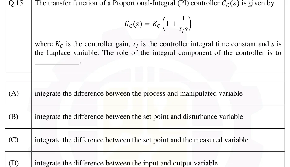
The transfer function of a Proportional-Integral (PI) controller $G_{C} (s)$ is given by

G_{C} (s) = K_{C} (1 + \frac{1}{τ _{I} s})

where $K_{C}$ is the controller gain, $τ_{I}$ is the controller integral time constant and $s$ is the Laplace variable. The role of the integral component of the controller is to ____________.

(A)
integrate the difference between the process and manipulated variable
(B)
integrate the difference between the set point and disturbance variable
(C)
integrate the difference between the set point and the measured variable
(D)
integrate the difference between the input and output variable

Answer and solution

GATE 2026 BT Q.15: answer and solution

See the question in the paper

Tap to open full size

GATE 2026 BT Q.15: answer and solution

GATE 2026 BT Q.36

GATE 2026 · BTQ.36 · 2 marks · MCQ

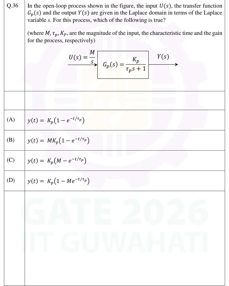
In the open-loop process shown in the figure, the input $U (s)$ , the transfer function $G_{p} (s)$ and the output $Y (s)$ are given in the Laplace domain in terms of the Laplace variable $s$ . For this process, which of the following is true?

(where $M, τ_{p}, K_{P}$ , are the magnitude of the input, the characteristic time and the gain for the process, respectively)

GATE 2026 BT question 36: Open-loop block diagram: an input arrow labelled U(s) = M/s enters a single rectangular block labelled G_p(s) = (K_p)/(τ_p… — Figure from the GATE 2026 BT paper. It is part of the question.

(A)
$y (t) = K_{p} (1 - e^{- t / τ_{p}})$
(B)
$y (t) = M K_{p} (1 - e^{- t / τ_{p}})$
(C)
$y (t) = K_{p} (M - e^{- t / τ_{p}})$
(D)
$y (t) = K_{p} (1 - M e^{- t / τ_{p}})$

Answer and solution

GATE 2026 BT Q.36: answer and solution

GATE 2025 BT Q.42

GATE 2025 · BTQ.42 · 2 marks · MCQ

A thermometer measuring body temperature follows a first-order response with a time constant of 40 seconds. The instrument will reach 95% of its steady-state output at __________ seconds.

(Round off to the nearest integer)

(A)
60
(B)
80
(C)
120
(D)
160

Answer and solution

GATE 2025 BT Q.42: answer and solution

See the question in the paper

Tap to open full size

GATE 2025 BT Q.42: answer and solution

GATE 2025 BT Q.43

GATE 2025 · BTQ.43 · 2 marks · MCQ

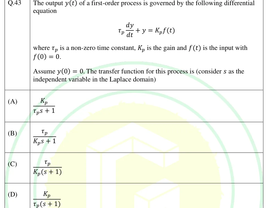
The output $y (t)$ of a first-order process is governed by the following differential equation

τ_{p} \frac{d y}{d t} + y = K_{p} f (t)

where $τ_{p}$ is a non-zero time constant, $K_{p}$ is the gain and $f (t)$ is the input with $f (0) = 0$ .

Assume $y (0) = 0$ . The transfer function for this process is (consider $s$ as the independent variable in the Laplace domain)

(A)
$\frac{K _{p}}{τ _{p} s + 1}$
(B)
$\frac{τ _{p}}{K _{p} s + 1}$
(C)
$\frac{τ _{p}}{K _{p} ( s + 1 )}$
(D)
$\frac{K _{p}}{τ _{p} ( s + 1 )}$

Answer and solution

GATE 2025 BT Q.43: answer and solution

See the question in the paper

Tap to open full size

GATE 2025 BT Q.43: answer and solution

GATE 2024 BT Q.12

GATE 2024 · BTQ.12 · 1 mark · MCQ

The transfer function of a process is $G (s) = \frac{K _{p}}{τ _{p} s + 1}$ , where $K_{p}$ is the gain and $τ_{p}$ is the time constant. This is a ________ process.

(A)
first order
(B)
multi-capacity
(C)
purely capacitive
(D)
second order

Answer and solution

GATE 2024 BT Q.12: answer and solution

See the question in the paper

Tap to open full size

GATE 2024 BT Q.12: answer and solution

GATE 2023 BT Q.64

GATE 2023 · BTQ.64 · 2 marks · NAT

A proportional controller is used to control the temperature of an autoclave from $60^{\circ} C$ to $130^{\circ} C$ . If the proportional band setting of the controller is 25%, the proportional gain value is __________.

Answer and solution

GATE 2023 BT Q.64: answer and solution

See the question in the paper

Tap to open full size

GATE 2023 BT Q.64: answer and solution

GATE 2022 BT Q.41

GATE 2022 · BTQ.41 · 2 marks · MCQ

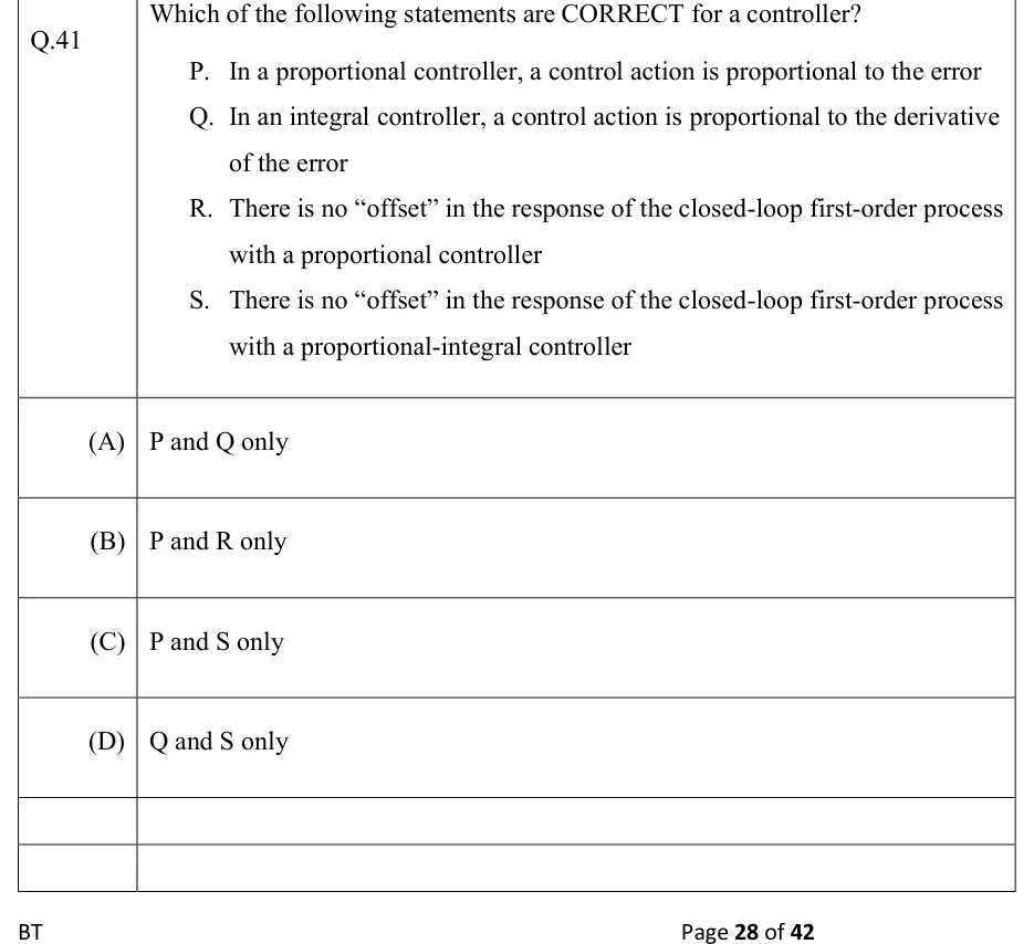
Which of the following statements are CORRECT for a controller?

P. In a proportional controller, a control action is proportional to the error

Q. In an integral controller, a control action is proportional to the derivative of the error

R. There is no "offset" in the response of the closed-loop first-order process with a proportional controller

S. There is no "offset" in the response of the closed-loop first-order process with a proportional-integral controller

(A)
P and Q only
(B)
P and R only
(C)
P and S only
(D)
Q and S only

Answer and solution

GATE 2022 BT Q.41: answer and solution

See the question in the paper

Tap to open full size

GATE 2022 BT Q.41: answer and solution

GATE 2019 BT Q.41

GATE 2019 · BTQ.41 · 2 marks · MCQ

Which one of the following statements is CORRECT about proportional controllers?

(A)
The initial change in control output signal is relatively slow
(B)
The initial corrective action is greater for larger error
(C)
They have no offset
(D)
There is no corrective action if the error is a constant

Answer and solution

GATE 2019 BT Q.41: answer and solution

See the question in the paper

Tap to open full size

GATE 2019 BT Q.41: answer and solution

GATE 2019 BT Q.42

GATE 2019 · BTQ.42 · 2 marks · MCQ

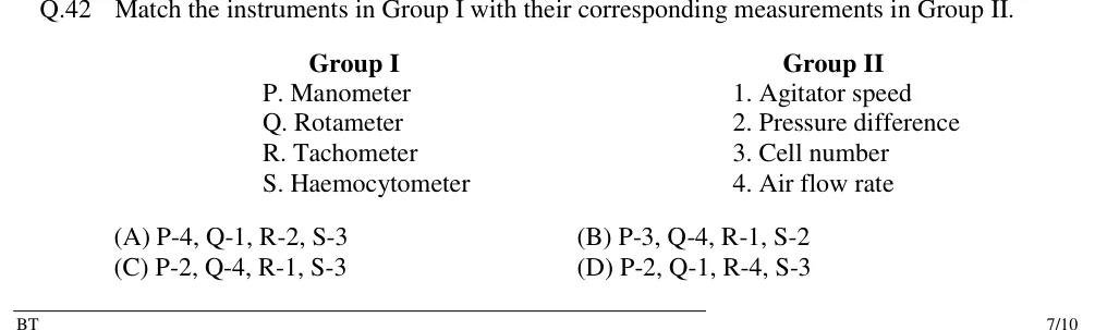
Match the instruments in Group I with their corresponding measurements in Group II.

| Group I | Group II |
|---|---|
| P. Manometer | 1. Agitator speed |
| Q. Rotameter | 2. Pressure difference |
| R. Tachometer | 3. Cell number |
| S. Haemocytometer | 4. Air flow rate |

(A)
P-4, Q-1, R-2, S-3
(B)
P-3, Q-4, R-1, S-2
(C)
P-2, Q-4, R-1, S-3
(D)
P-2, Q-1, R-4, S-3

Answer and solution

GATE 2019 BT Q.42: answer and solution

See the question in the paper

Tap to open full size

GATE 2019 BT Q.42: answer and solution

PRACTICE

6 questions to test yourself

PRACTICE 11 mark · MCQ

The jacket of an exothermic fermentation is cooled by water supplied through an air-to-close (fail-open) control valve. The temperature transmitter has a positive gain, and the controller error is defined as $e = T_{s p} - T_{m}$ . For the temperature loop to provide negative feedback, the controller must be

(A)
reverse acting ( $K_{c} > 0$ )
(B)
direct acting ( $K_{c} < 0$ )
(C)
reverse acting for set-point changes and direct acting for load changes
(D)
of either action, because the loop is stable for either sign of $K_{c}$

Answer and solution

Answer: (A)

Air-to-close valve: a higher controller output closes the valve, so $K_{v} < 0$ .
More cooling water lowers the broth temperature, so $K_{p} < 0$ . The transmitter has $K_{m} > 0$ .
Negative feedback needs $K_{c} K_{v} K_{p} K_{m} > 0$ . Since $K_{v} K_{p} K_{m} > 0$ , $K_{c} > 0$ : a reverse-acting controller.
Check: if $T$ rises, $e$ falls, the output falls, the air-to-close valve opens, and more cooling brings $T$ back down.

PRACTICE 21 mark · NAT

A thermometer behaves as a first-order system with unit gain and a time constant of 12 s. It reads a steady 30 °C, and at $t = 0$ it is plunged into a well-stirred bath held at 80 °C. Its reading (in °C) at $t = 18$ s is ________ (round off to two decimal places).

Answer and solution

Answer: $68.84$ (accepted range $\pm 0.1$ )

Step of 50 °C into $1/ (12 s + 1)$ : $T (t) = 30 + 50 (1 - e^{- t /12})$ .
At $t = 18$ s: $e^{- 1.5} = 0.2231$ , so $T = 30 + 50 \times 0.7769 = 68.84$ °C.

PRACTICE 32 marks · NAT

A fermenter temperature loop uses a proportional-only controller with gain $K_{c} > 0$ . In consistent deviation units, with time in minutes, $G_{v} = G_{m} = 1$ , $G_{p} (s) = \frac{2}{10 s + 1}$ , and a disturbance $d$ acts on the temperature through $G_{d} (s) = \frac{0.5}{10 s + 1}$ . The set point is held constant. The minimum controller gain $K_{c}$ for which a step of magnitude 4 in $d$ leaves a steady-state offset of magnitude no more than 0.1 is ________ (round off to one decimal place).

Answer and solution

Answer: $9.5$ (accepted range $\pm 0.05$ )

Regulator problem: $\frac{Y}{D} = \frac{G _{d}}{1 + K _{c} G _{p}} = \frac{0.5/ ( 10 s + 1 )}{1 + 2 K _{c} / ( 10 s + 1 )} = \frac{0.5}{10 s + 1 + 2 K _{c}}$ . With $K_{c} > 0$ the single pole $s = - (1 + 2 K_{c}) /10$ is negative, so the loop is stable and the final value theorem applies.
Final value for $D = 4/ s$ : $y (\infty) = lim_{s \to 0} s \cdot \frac{0.5}{10 s + 1 + 2 K _{c}} \cdot \frac{4}{s} = \frac{2}{1 + 2 K _{c}}$ .
Since the set point is unchanged, the offset has magnitude $2/ (1 + 2 K_{c})$ . Setting $2/ (1 + 2 K_{c}) \leq 0.1$ gives $1 + 2 K_{c} \geq 20$ , so $K_{c} \geq 9.5$ .

PRACTICE 41 mark · NAT

A process has transfer function $G (s) = \frac{9}{s ^{2} + 1.2 s + 9}$ . Starting from steady state, its input is stepped up by 2 units. The maximum value reached by the output deviation is ________ (round off to two decimal places).

Answer and solution

Answer: $3.05$ (accepted range $\pm 0.02$ )

Divide by 9: $G = \frac{1}{s ^{2} /9 + 0.1333 s + 1}$ , so $K = 1$ , $τ = 1/3$ , and $2 ζ τ = 0.1333$ gives $ζ = 0.2$ .
Overshoot $= exp (- π \times 0.2/ 0.96) = exp (- 0.6413) = 0.5266$ .
Final change $= K M = 2$ . Maximum value $= 2 (1 + 0.5266) = 3.05$ .

PRACTICE 52 marks · NAT

A feedback loop has open-loop transfer function $G_{O L} (s) = \frac{4 K _{c}}{( 5 s + 1 ) ( 2 s + 1 ) ( s + 1 )}$ , with time in minutes, where $K_{c}$ is the gain of a controller. Using the Ziegler–Nichols ultimate-gain (continuous cycling) settings, the controller gain $K_{c}$ for a PI controller is ________ (round off to two decimal places).

Answer and solution

Answer: $1.42$ (accepted range $\pm 0.02$ )

$(5 s + 1) (2 s + 1) (s + 1) = 10 s^{3} + 17 s^{2} + 8 s + 1$ , so the characteristic equation is $10 s^{3} + 17 s^{2} + 8 s + 1 + 4 K_{c} = 0$ .
Cubic Routh condition: $17 \times 8 > 10 (1 + 4 K_{c})$ , i.e. $136 > 10 + 40 K_{c}$ , so $K_{c} < 3.15$ and $K_{u} = 3.15$ .
At $K_{u}$ : $ω_{u}^{2} = a_{2} / a_{0} = 8/10$ , so $ω_{u} = 0.894$ rad/min and $P_{u} = 2 π /0.894 = 7.02$ min (giving $τ_{I} = P_{u} /1.2 = 5.85$ min).
ZN PI gain: $K_{c} = 0.45 K_{u} = 0.45 \times 3.15 = 1.4175$ , which rounds to 1.42.

PRACTICE 62 marks · MSQ

Which of the following statements is/are correct?

(A)
At constant pressure drop, an equal-percentage valve with rangeability 50 passes about 14% of its maximum flow at half stem travel.
(B)
A feed-forward controller used on its own corrects for disturbances that are not measured.
(C)
Adding a feed-forward controller to an existing feedback loop does not change the roots of the closed-loop characteristic equation.
(D)
Adding derivative action to a proportional-only controller removes the steady-state offset for a step change in set point.

Answer and solution

Answer: (A), (C)

A: $f = R^{x - 1} = 5 0^{- 0.5} = 0.141$ , i.e. about 14%. Correct.
B: feed-forward acts only on the disturbance it measures and has no feedback of the output, so unmeasured disturbances go uncorrected. Incorrect.
C: the feed-forward block acts on the measured disturbance, outside the feedback loop, so $1 + G_{c} G_{v} G_{p} G_{m} = 0$ is unchanged. Correct.
D: at steady state $d e / d t = 0$ , so derivative action contributes nothing and a PD controller leaves the same offset as P. Incorrect.

OFFICIAL GATE 2027 SYLLABUS WORDING

Copied from the GATE 2027 syllabus; see all 2027 syllabi.

GATE BT

Measurement devices; Valves; First order and second order systems; Feedback and feed forward control; Types of controllers – proportional, derivative and integral control; Tuning of controllers

Preparing in Kolkata? IAE Academy's course for GATE BT.