IN THE IN SYLLABUS

Actuators, time delay and industrial control

Real plants add dead time to their loops, and every controller output reaches the process through a valve or motor whose characteristic and transfer function shape the loop. A pure delay removes phase margin without touching the magnitude plot, and a valve's characteristic changes the loop gain as the flow changes. These notes cover delay-margin and Pade–Routh stability calculations, the Smith predictor, valve characteristics, $C_{v}$ sizing and fail-safe choice, servo-valve, DC and AC servo-motor and stepper-motor formulas, cascade, feedforward and ratio control, and how supervisory control, PLC scans, ladder logic, timers, DCS and SCADA work.

2 previous-year questions · 2 solved · 7 practice questions

Dead time (transport lag) and FOPDT models

A pure time delay of $T$ seconds passes a signal through unchanged but late. For a signal $x (t)$ that is zero for $t < 0$ , the output is $y (t) = x (t - T) u (t - T)$ , so $Y (s) = e^{- s T} X (s)$ . It appears whenever material or information has to travel before it is measured or takes effect. Examples are fluid moving along a pipe to a sensor, a conveyor carrying solids, an analyser's sample line, and a digital controller's computation and communication time. The delay is not a ratio of polynomials and has no finite poles or zeros. Once it sits inside a feedback loop, the characteristic equation $1 + G (s) H (s) e^{- s T} = 0$ is transcendental and has infinitely many roots.

FREQUENCY RESPONSE OF A PURE DELAY

e^{- j ω T} = 1, ∠ e^{- j ω T} = - ω T rad = - \frac{18 0 ^{\circ}}{π} ω T

Holds at every $ω$ ( $ω$ in rad/s, $T$ in s). The magnitude plot is untouched. The phase lag grows linearly with $ω$ , so on a logarithmic frequency axis it falls away more and more steeply.

Three consequences follow directly. (1) The gain-crossover frequency $ω_{g c}$ does not move, because the magnitude does not change. (2) The phase margin falls by $ω_{g c} T$ radians. (3) The phase crossover moves to a lower frequency, and a loop whose phase never reached $- 18 0^{\circ}$ now gets a phase crossover. When $∣ G H ∣$ decreases with frequency, the magnitude at the new, lower phase crossover is larger, so the gain margin falls too. A loop that was stable for every gain without delay (for example a first- or second-order type-0 plant, or a pure integrator, under proportional control) now has a finite ultimate gain. On the Nyquist plot, every point $G (j ω) H (j ω)$ is rotated clockwise by $ω T$ radians. A strictly proper plot therefore spirals into the origin and crosses the negative real axis infinitely often.

PHASE MARGIN WITH AN ADDED DELAY

P M_{T} = P M_{0} - \frac{18 0 ^{\circ}}{π} ω_{g c} T, P M_{0} = 18 0^{\circ} + ∠ G (j ω_{g c}) H (j ω_{g c})

$P M_{0}$ is the margin of the delay-free loop and $ω_{g c}$ is its gain-crossover frequency (where $∣ G H ∣ = 1$ ). This is valid because the delay leaves $ω_{g c}$ where it was. Read stability from $P M_{T} > 0$ only when the magnitude crosses 0 dB once and the open loop has no right-half-plane poles.

DELAY MARGIN (LARGEST TOLERABLE DEAD TIME)

T_{m a x} = \frac{P M _{0} ( in rad )}{ω _{g c}}

$P M_{0}$ is the phase margin of the delay-free loop, so $T_{m a x}$ is the TOTAL loop delay at which the phase margin reaches zero and the closed loop becomes marginally stable. Convert the margin to radians first. If the loop already contains a delay $T_{0}$ , the extra delay it can tolerate is $T_{m a x} - T_{0}$ , which equals (present phase margin in rad) $/ ω_{g c}$ . Assumes the delay-free closed loop is stable ( $P M_{0} > 0$ ) and the magnitude crosses 0 dB only once.

INTEGRATOR PLUS DEAD TIME

G (s) H (s) = \frac{K e ^{- s T}}{s} is closed-loop stable ⟺ 0 < K T < \frac{π}{2}

Negative feedback, $K > 0$ , $T > 0$ . The gain crossover is at $ω_{g c} = K$ , where the phase margin is $π /2 - K T$ rad. The phase crossover is where $π /2 + ω T = π$ , i.e. $ω_{p c} = π / (2 T)$ , and there $∣ G H ∣ = 2 K T / π$ . Equivalently, the delay margin is $T_{m a x} = π / (2 K)$ .

ULTIMATE GAIN AND FREQUENCY WITH DEAD TIME

∠ G_{0} (j ω_{u}) - ω_{u} T = - π, K_{u} = \frac{1}{∣ G _{0} ( j ω _{u} ) ∣}

For the loop $K G_{0} (s) e^{- s T}$ under negative feedback, $K > 0$ . Solve the phase condition (usually by trial) for its lowest root $ω_{u}$ in rad/s, then read off $K_{u}$ : the gain at which the closed loop is marginally stable and oscillates at $ω_{u}$ . Valid when $G_{0}$ has no right-half-plane poles and $∣ G_{0} (j ω) ∣$ decreases with frequency. The Pade example in the next section works one out exactly.

Most overdamped industrial processes, such as a tank, a heat exchanger or a chain of lags, are modelled from a step test as first order plus dead time (FOPDT). The apparent dead time also absorbs the small extra lags of a higher-order process.

FIRST-ORDER-PLUS-DEAD-TIME (FOPDT) MODEL

G (s) = \frac{K e ^{- θ s}}{τ s + 1}, ∠ G (j ω) = - tan^{- 1} (ω τ) - ω θ rad

$K$ = steady-state gain, $τ$ = time constant, $θ$ = dead time. The ratio $θ / τ$ measures how hard the process is to control: the larger it is, the smaller the loop gain $K K_{c}$ at which a proportional loop becomes unstable.

FOPDT STEP RESPONSE (INPUT STEP OF SIZE A)

y (t) = 0 (t < θ), y (t) = K A (1 - e^{- (t - θ) / τ}) (t \geq θ)

Nothing happens for $θ$ seconds. After that the response is an ordinary first-order rise, reaching 63.2% of $K A$ at $t = θ + τ$ .

TWO-POINT FOPDT FIT FROM A STEP TEST

τ = 1.5 (t_{63.2} - t_{28.3}), θ = t_{63.2} - τ, K = \frac{Δ y _{\infty}}{Δ u}

$t_{28.3}$ and $t_{63.2}$ are the times at which the response has completed 28.3% and 63.2% of its final change. The fit works because $1 - e^{- 1/3} = 0.283$ and $1 - e^{- 1} = 0.632$ , so those points fall at $θ + τ /3$ and $θ + τ$ .

WORKED EXAMPLE

A unity-feedback loop has open-loop transfer function $G (s) = \frac{15 e ^{- 0.1 s}}{s ( s + 4 )}$ . Find (a) the phase margin and (b) the total dead time at which the closed loop becomes marginally stable.

Solution

Magnitude (the delay contributes a factor of 1): $∣ G (j ω) ∣ = \frac{15}{ω ω ^{2} + 16}$ . At $ω = 3$ this is $15/ (3 \times 5) = 1$ . The magnitude falls monotonically, so $ω_{g c} = 3$ rad/s is the only crossover.
Delay-free phase at $ω_{g c}$ : $- 9 0^{\circ} - tan^{- 1} (3/4) = - 9 0^{\circ} - 36.8 7^{\circ} = - 126.8 7^{\circ}$ , so $P M_{0} = 18 0^{\circ} - 126.8 7^{\circ} = 53.1 3^{\circ}$ .
Phase added by the delay at $ω_{g c}$ : $- ω_{g c} T = - 3 \times 0.1 = - 0.3$ rad $= - 17.1 9^{\circ}$ .
(a) $P M = 53.1 3^{\circ} - 17.1 9^{\circ} = 35.9 4^{\circ}$ . It is positive and there is one crossover, so the loop is stable.
(b) $P M_{0} = 53.1 3^{\circ} = 0.9273$ rad, so the total delay limit is $T_{m a x} = 0.9273/3 = 0.309$ s. Check: the present margin $35.9 4^{\circ} = 0.6273$ rad gives an extra $0.6273/3 = 0.209$ s, and $0.1 + 0.209 = 0.309$ s.

Answer: (a) $P M \approx 35. 9^{\circ}$ . (b) The loop becomes marginally stable when the total dead time reaches about 0.309 s, i.e. about 0.21 s more than it has now.

EXAM TIP

Degrees and radians: the delay's phase $ω T$ comes out in radians. Multiply it by $180/ π \approx 57.3$ before subtracting it from a margin in degrees. For the delay margin, convert the margin to radians before dividing by $ω_{g c}$ .

EXAM TIP

A delay never changes the magnitude plot, the gain-crossover frequency or the steady-state gain ( $e^{0} = 1$ ), so the static error constants $K_{p}$ , $K_{v}$ , $K_{a}$ are unchanged too, provided the closed loop stays stable. Reject any option that says a delay changes them.

Sampled-data loops: if the delay is an exact multiple of the sampling period, $T = N T_{s}$ , it becomes $z^{- N}$ in the z-domain. That is a rational function, so the z-domain characteristic equation is an ordinary polynomial (of higher order) and the usual discrete stability tests apply directly.

Stability with dead time: Pade approximation and the Smith predictor

Routh–Hurwitz needs a polynomial, so it cannot be applied to $1 + G (s) e^{- s T} = 0$ directly. There are two routes. The frequency-response route (Bode or Nyquist, using the exact phase $- ω T$ ) is exact. The algebraic route replaces $e^{- s T}$ with a rational Pade approximation and then applies Routh; it is quick but approximate.

FIRST-ORDER PADE APPROXIMATION

e^{- s T} \approx \frac{1 - \frac{s T}{2}}{1 + \frac{s T}{2}} = \frac{2 - s T}{2 + s T}

An all-pass: magnitude exactly 1, phase $- 2 tan^{- 1} (ω T /2)$ . It puts a right-half-plane zero at $s = + 2/ T$ (non-minimum phase) and a pole at $s = - 2/ T$ . Accurate while $ω T$ is well below 1.

SECOND-ORDER PADE APPROXIMATION

e^{- s T} \approx \frac{1 - \frac{s T}{2} + \frac{s ^{2} T ^{2}}{12}}{1 + \frac{s T}{2} + \frac{s ^{2} T ^{2}}{12}}

Also all-pass, with two right-half-plane zeros (a complex pair). It follows the true phase to higher frequencies than the first-order form.

SERIES (LAG) APPROXIMATIONS

e^{- s T} \approx 1 - s T or e^{- s T} \approx \frac{1}{1 + s T}

First-order Taylor forms, valid only for small $s T$ . The lag form is how a small delay gets lumped into an extra time constant. Neither form has unit magnitude, so use Pade for stability work.

EXAM TIP

Pade under-estimates phase lag. Since $tan^{- 1} y < y$ for $y > 0$ , the first-order Pade lag $2 tan^{- 1} (ω T /2)$ is always smaller than the true $ω T$ . For a plant whose magnitude falls with frequency, a stability limit computed with Pade is therefore optimistic (too large), as the example below shows.

WORKED EXAMPLE

A unity-feedback loop has $G (s) = \frac{K e ^{- s}}{s + 1}$ with $K > 0$ . Estimate the largest stable $K$ using the first-order Pade approximation, and compare it with the exact value.

Solution

Pade with $T = 1$ : $e^{- s} \approx \frac{2 - s}{2 + s}$ .
Characteristic equation: $(s + 1) (s + 2) + K (2 - s) = 0 \Rightarrow s^{2} + (3 - K) s + (2 + 2 K) = 0$ .
A second-order polynomial is stable if and only if all its coefficients have the same sign. So $3 - K > 0$ and $2 + 2 K > 0$ , giving $- 1 < K < 3$ . Estimate: $K_{m a x} = 3$ . At $K = 3$ the equation is $s^{2} + 8 = 0$ , an oscillation at $2.83$ rad/s.
Exact: the phase crossover satisfies $tan^{- 1} ω + ω = π$ . By trial, $ω = 2$ gives $3.107$ rad and $ω = 2.03$ gives $3.143$ rad, so $ω_{p c} \approx 2.03$ rad/s.
Setting $∣ G (j ω_{p c}) ∣ = 1$ : exact $K_{m a x} = 1 + ω_{p c}^{2} = 1 + 2.0 3^{2} \approx 2.26$ .

Answer: The Pade estimate is $K_{m a x} = 3$ (oscillation at 2.83 rad/s). The exact value is $K_{m a x} \approx 2.26$ (at 2.03 rad/s), so the first-order Pade estimate is about 33% too high.

Dead-time compensation (Smith predictor). Let the plant be $G_{p} (s) = G_{0} (s) e^{- θ s}$ . If the controller holds a model of it, it can predict what the output will be once the delay has passed. The controller output is passed through the model $G_{0} (s) (1 - e^{- θ s})$ , and the result is added to the measured output before it is compared with the setpoint. This local path wraps $G_{c}$ in negative feedback and gives the equivalent controller $\frac{G _{c}}{1 + G _{c} G _{0} ( 1 - e ^{- θ s} )}$ .

SMITH PREDICTOR WITH A PERFECT MODEL

\frac{Y ( s )}{R ( s )} = \frac{G _{c} ( s ) G _{0} ( s )}{1 + G _{c} ( s ) G _{0} ( s )} e^{- θ s}

The delay leaves the characteristic equation, so $G_{c}$ can be tuned as if the plant had no dead time. The output is the delay-free response shifted by $θ$ . If the model of $G_{0}$ or $θ$ is wrong, the delay comes back into the characteristic equation.

EXAM TIP

No controller can remove the dead time from the setpoint response: the output still starts moving $θ$ seconds after the setpoint changes. A Smith predictor takes the delay out of the characteristic equation, so it no longer limits the controller gain. It depends on an accurate model of both $G_{0}$ and $θ$ .

Control valves: characteristics, sizing and fail-safe action

A pneumatic control valve has a body (plug and seat, or a ball or butterfly), a spring-and-diaphragm actuator, and often a positioner that closes a local loop on stem position. An I/P transducer converts the electronic controller's 4–20 mA output to the standard 3–15 psi air signal (metric 20–100 kPa, about 0.2–1.0 bar), which moves the stem against the spring. Below, $x$ is the fractional stem travel (0 closed, 1 fully open) and $f = q / q_{m a x}$ is the fractional flow.

SPRING-AND-DIAPHRAGM ACTUATOR

\frac{X _{s} ( s )}{P ( s )} = \frac{A}{M s ^{2} + b s + k}, x_{s, ss} = \frac{A p}{k}

Force balance on the stem. $A$ = diaphragm area, $p$ = signal pressure measured from the pressure at which the stem starts to move (the spring preload, 3 psi for a full-range 3–15 psi valve), $k$ = spring stiffness, $M$ = moving mass, $b$ = viscous friction coefficient. Static friction and fluid forces on the plug are neglected. The mass is usually small, so the actuator is often reduced to a first-order lag or a pure gain.

INHERENT CHARACTERISTICS (CONSTANT PRESSURE DROP ACROSS THE VALVE)

Linear: f = x Equal percentage: f = R^{x - 1} Quick opening: f \approx x

$R$ is the rangeability. The ideal equal-percentage law gives $f = 1/ R$ at $x = 0$ , so it never reaches zero; the real valve shuts by seating. The square-root law is one common model of quick opening.

EQUAL-PERCENTAGE GAIN

\frac{df}{d x} = f ln R \Rightarrow \frac{1}{f} \frac{df}{d x} = ln R, \frac{f ( x + Δ x )}{f ( x )} = R^{Δ x}

Equal steps of travel change the current flow by equal percentages. The gain is proportional to flow: small near closed, large near fully open.

RANGEABILITY

R = \frac{q _{m a x}}{q _{m i n}} (controllable flows)

Ratio of the largest to the smallest flow the valve can control. For the ideal equal-percentage valve, $R = f (1) / f (0)$ .

VALVE FLOW COEFFICIENT (LIQUIDS)

q = C_{v} f (x) \frac{Δ P}{G}

$q$ in US gal/min, $Δ P$ across the valve in psi, $G$ = specific gravity relative to water. $C_{v}$ is the water flow in gal/min through the fully open valve ( $f = 1$ ) at a 1 psi drop. The metric coefficient $K_{v}$ uses m³/h and bar, with $C_{v} \approx 1.156 K_{v}$ .

INSTALLED CHARACTERISTIC

\frac{q}{q _{m a x}} = \frac{f ( x )}{β + ( 1 - β ) f ( x ) ^{2}}, β = \frac{Δ P _{valve, fully open}}{Δ P _{total}}

Applies when a fixed total pressure drop is shared between the valve and a line resistance whose drop is $\propto q^{2}$ . Here $q_{m a x}$ is the flow with the valve fully open in this installation. The valve authority $β = 1$ gives the inherent curve. As $β$ falls, a linear valve behaves more like quick opening and an equal-percentage valve moves toward linear.

SIGNAL TO TRAVEL (FULL-RANGE CALIBRATION)

ATO: x = \frac{I - 4}{16}, ATC: x = \frac{20 - I}{16}, I in mA

In terms of air pressure: $x = (p - 3) /12$ for $p$ in psi on an air-to-open valve.

For loop analysis, the valve, actuator and positioner together are modelled as a gain $K_{v}$ , often with a first-order lag $K_{v} / (τ_{v} s + 1)$ . $K_{v}$ is the slope of the installed characteristic at the operating point times $d x / d I$ . For a linear valve at constant pressure drop, $K_{v}$ is constant. For an equal-percentage valve it is proportional to the flow, as the example below shows.

Inherent characteristic	Law	Gain $df / d x$	Typical use
Linear	$f = x$	Constant (1)	The valve takes most of the system pressure drop, so the installed curve stays close to the inherent one. Level and flow loops with roughly constant process gain
Equal percentage	$f = R^{x - 1}$	$f ln R$ , rises with flow	The valve takes a small share of the drop (the installed curve moves toward linear), or the process gain falls as load rises. Temperature and pressure loops
Quick opening	$f \approx x$	Large near closed, small near open	On/off service, and safety and relief duties that need full flow after little travel

Actuator action	Rising signal	On loss of air or signal	Choose it when the safe state is
Air-to-open (ATO)	Opens the valve	Spring closes it: fail-closed (FC)	No flow, e.g. fuel gas to a furnace, steam to a heater, feed to a reactor
Air-to-close (ATC)	Closes the valve	Spring opens it: fail-open (FO)	Full flow, e.g. cooling water to an exothermic reactor, a vent or relief line

The valve action fixes the sign of the valve gain: positive for ATO, negative for ATC. The controller's direct or reverse action is then chosen so that the product of all the gains around the loop gives negative feedback. If nothing else in the loop changes, switching a valve from ATO to ATC means reversing the controller action.

WORKED EXAMPLE

An equal-percentage valve with rangeability $R = 50$ passes $q_{m a x} = 100$ m³/h at constant pressure drop. It is air-to-open and driven by a 4–20 mA signal through a linear I/P and actuator. Find (a) the flow at 10.4 mA, (b) the valve gain there in (m³/h)/mA, and (c) the percentage change in flow for a further 10% of travel.

Solution

$x = (10.4 - 4) /16 = 0.4$ .
(a) $f = 5 0^{0.4 - 1} = 5 0^{- 0.6} = e^{- 0.6 l n 50} = e^{- 2.347} = 0.0956$ , so $q = 9.56$ m³/h.
(b) $\frac{d q}{d x} = q ln R = 9.56 \times 3.912 = 37.4$ m³/h per unit travel. With $d x / d I = 1/16$ per mA, the gain is $37.4/16 = 2.34$ (m³/h)/mA.
(c) $Δ x = 0.1$ multiplies the flow by $5 0^{0.1} = e^{0.391} = 1.479$ . That is a 47.9% increase, whatever the starting point.
For comparison, a linear valve at 10.4 mA would pass 40 m³/h with a constant gain of $100/16 = 6.25$ (m³/h)/mA.

Answer: (a) 9.56 m³/h; (b) about 2.34 (m³/h)/mA; (c) +47.9%.

EXAM TIP

$q \propto Δ P$ at a fixed opening: four times the pressure drop gives twice the flow, not four times. $C_{v}$ is defined at full opening; at partial opening, multiply by $f (x)$ .

EXAM TIP

Fail-safe action is chosen for process safety, never for control performance. Choose it first, then set the controller action to match.

EXAM TIP

The inherent characteristic assumes a constant $Δ P$ across the valve (a test-bench curve). The installed characteristic is the valve in its piping, where $Δ P$ falls as flow rises. A question that gives a line pressure drop is asking about the installed curve.

Servo valves, servo motors and stepper motors

An electro-hydraulic servo valve turns a small input current into a proportional flow of high-pressure oil. A torque motor deflects a flapper between two nozzles (or swings a jet pipe). The resulting pressure difference shifts the main spool, and a feedback spring re-centres the flapper so that spool displacement is proportional to the current. Oil flow to the actuator is then proportional to spool displacement at a given load pressure. The valve's own dynamics are usually modelled as first order, $K_{s v} / (τ_{s v} s + 1)$ , or as second order. Hydraulics give very high force for their size and a fast response, so they drive aircraft control surfaces, machine-tool slides, turbine governors and large valves.

SERVO-VALVE FLOW, LINEARISED

q_{L} = K_{q} x_{v} - K_{c} p_{L}

$x_{v}$ = spool displacement ( $\propto$ input current), $p_{L}$ = load pressure difference, $K_{q}$ = flow gain, $K_{c}$ = flow–pressure coefficient (how much the flow drops as load pressure rises).

VALVE-CONTROLLED HYDRAULIC PISTON

q_{L} = A \frac{d y}{d t} \Rightarrow \frac{Y ( s )}{X _{v} ( s )} = \frac{K _{q}}{A s}

Piston area $A$ . Neglects the load-pressure term $K_{c} p_{L}$ (no load), oil compressibility and leakage. The actuator is then an integrator, so a unity-feedback position loop with a proportional controller is type 1 and has zero steady-state error to a step command.

DC servo motors. In armature control, the field current is held constant and the armature voltage $V_{a}$ is the input. The back emf $e_{b} = K_{b} ω$ feeds back inside the motor and acts as electrical damping. In field control, the armature current is held constant and the field voltage is the input, so there is no back-emf feedback.

ARMATURE-CONTROLLED DC MOTOR

\frac{θ ( s )}{V _{a} ( s )} = \frac{K _{t}}{s [ ( R _{a} + L _{a} s ) ( J s + B ) + K _{t} K _{b} ]}

$K_{t}$ = torque constant (N·m/A), $K_{b}$ = back-emf constant (V·s/rad); the two are numerically equal in SI units. $J$ and $B$ are the total inertia and viscous friction referred to the motor shaft. Speed is $ω (s) = s θ (s)$ .

ARMATURE CONTROL, ARMATURE INDUCTANCE NEGLECTED

\frac{θ ( s )}{V _{a} ( s )} = \frac{K _{m}}{s ( τ _{m} s + 1 )}, K_{m} = \frac{K _{t}}{R _{a} B + K _{t} K _{b}}, τ_{m} = \frac{R _{a} J}{R _{a} B + K _{t} K _{b}}

$K_{m}$ in (rad/s)/V is the steady-state speed per volt. Back emf shortens the time constant from $J / B$ to $τ_{m}$ .

FIELD-CONTROLLED DC MOTOR

\frac{θ ( s )}{V _{f} ( s )} = \frac{K _{t f}}{s ( R _{f} + L _{f} s ) ( J s + B )}

Armature current is constant and the torque is $T = K_{t f} i_{f}$ . With no back-emf feedback there is no electrical damping, and the field time constant $L_{f} / R_{f}$ is significant. Used for small motors.

TWO-PHASE AC SERVO MOTOR

T = K_{1} e_{c} - K_{2} ω, \frac{θ ( s )}{E _{c} ( s )} = \frac{K _{m}}{s ( τ _{m} s + 1 )}, K_{m} = \frac{K _{1}}{B + K _{2}}, τ_{m} = \frac{J}{B + K _{2}}

The reference winding has a fixed voltage, and the control-winding voltage $e_{c}$ is 90° out of phase with it. $K_{1}$ = stall torque per volt of $e_{c}$ . $K_{2}$ = magnitude of the slope of the torque–speed line (stall torque ÷ no-load speed), which acts like extra viscous friction. The rotor has a high resistance-to-reactance ratio so that this line slopes downward over the whole speed range.

Stepper motors turn through a fixed angle for each input pulse. The number of pulses sets the position and the pulse rate sets the speed, so they can position in open loop with no feedback sensor. As long as no step is missed, the position error does not build up from step to step, and an energised motor holds its position (holding torque). Steps are lost if the load torque or the stepping rate exceeds what the motor can follow, and an open-loop drive cannot detect this. Two torque–rate curves describe the limit. The pull-in curve gives the largest load torque at which the motor can start, stop or reverse in step with the pulses at a given rate. The pull-out curve gives the largest load torque it can drive once it is already running at that rate. The pull-out curve lies above the pull-in curve, and the region between them is the slew range, which is reached only by ramping the pulse rate up and down. Microstepping divides each full step electronically by driving proportioned currents in two phases, giving finer resolution and smoother motion.

STEP ANGLE, VARIABLE RELUCTANCE (FULL STEP, ONE PHASE ON)

β = \frac{36 0 ^{\circ}}{m N _{r}} = \frac{N _{s} - N _{r}}{N _{s} N _{r}} \times 36 0^{\circ}

$m$ = number of stator phases, $N_{r}$ = rotor teeth, $N_{s}$ = stator teeth (poles). The two forms agree for the usual designs, where $N_{s} - N_{r} = N_{s} / m$ .

STEP ANGLE, HYBRID

β = \frac{36 0 ^{\circ}}{2 m N _{r}}

Two phases and 50 rotor teeth give $1. 8^{\circ}$ , i.e. 200 steps per revolution.

RESOLUTION AND SPEED

S = \frac{36 0 ^{\circ}}{β} steps/rev, n = \frac{β f}{6} rpm

$f$ = stepping rate in steps (pulses) per second, $β$ in degrees. Half-step drive halves $β$ and doubles $S$ .

Type	Rotor	Detent torque when unenergised	Step angle
Variable reluctance	Toothed soft iron, no magnet	None	$36 0^{\circ} / (m N_{r})$ ; moderate
Permanent magnet	Magnetised, no teeth	Yes	$36 0^{\circ} / (m P_{r})$ with $P_{r}$ rotor poles; large
Hybrid	Toothed and axially magnetised	Yes	$36 0^{\circ} / (2 m N_{r})$ ; small

WORKED EXAMPLE

An armature-controlled DC servo motor has $R_{a} = 2 Ω$ , negligible $L_{a}$ , $K_{t} = K_{b} = 0.5$ (SI units), $J = 0.02$ kg·m² and $B = 0.01$ N·m·s/rad. Find its transfer function $θ (s) / V_{a} (s)$ and its steady-state speed for a constant 12 V input.

Solution

$R_{a} B + K_{t} K_{b} = 2 (0.01) + 0.5 (0.5) = 0.02 + 0.25 = 0.27$ .
$K_{m} = 0.5/0.27 = 1.85$ (rad/s)/V and $τ_{m} = R_{a} J /0.27 = 0.04/0.27 = 0.148$ s.
So $\frac{θ ( s )}{V _{a} ( s )} = \frac{1.85}{s ( 0.148 s + 1 )}$ .
Steady-state speed $= K_{m} \times 12 = 22.2$ rad/s $= 22.2 \times 60/ (2 π) \approx 212$ rpm.
Without back emf the time constant would be $J / B = 2$ s. The electrical damping $K_{t} K_{b} / R_{a} = 0.125$ N·m·s/rad is 12.5 times the viscous friction, which is why $τ_{m}$ is so much shorter.

Answer: $θ (s) / V_{a} (s) = 1.85/ [s (0.148 s + 1)]$ ; about 22.2 rad/s (212 rpm) at 12 V.

EXAM TIP

$K_{t} = K_{b}$ only when both are in SI units (N·m/A and V·s/rad). If $K_{b}$ is given in V per 1000 rpm, convert it before using it as $K_{t}$ .

EXAM TIP

An ordinary induction motor has a low rotor resistance, which gives its torque–speed curve a region of positive slope, and that region would make a servo loop unstable. AC servo motors use high-resistance rotors to avoid it.

EXAM TIP

For stepper speed questions, first find the step angle for the stated drive mode (full or half step), then use $n = β f /6$ rpm. Equivalently, $n = 60 f / S$ .

Cascade, feedforward and ratio control

Cascade control uses two controllers and two measurements but only one manipulated variable. The primary (master, outer) controller acts on the variable that matters. Its output becomes the setpoint of the secondary (slave, inner) controller, which drives the valve. In a jacketed reactor, for example, reactor temperature is the primary variable and jacket temperature (or coolant flow) is the secondary. A disturbance in the coolant supply upsets the jacket first, and the fast inner loop corrects it before the reactor temperature moves.

The secondary variable must be measurable, must respond to the manipulated variable, and must be affected by the disturbance you want rejected (that disturbance enters the inner loop).
The inner loop must be clearly faster than the outer loop, by several times. Otherwise cascade gives little benefit and the two loops interact.
Inner controller: P or PI (the outer loop's integral action removes any small inner offset). Outer controller: PI or PID.
Tune the inner loop first, with the outer loop in manual. Then switch the inner controller to cascade (remote setpoint) and tune the outer loop.
The inner loop also encloses the valve, so the effect of valve nonlinearity (a valve gain that changes with opening) is largely compensated inside it.
Cascade adds a measurement and a controller, not an actuator: there is still one valve.

CASCADE LOOP, INNER LOOP REDUCED FIRST

G_{2}^{c l} = \frac{G _{c 2} G _{v} G _{p 2}}{1 + G _{c 2} G _{v} G _{p 2} H _{2}}, \frac{Y _{1}}{R _{1}} = \frac{G _{c 1} G _{2}^{c l} G _{p 1}}{1 + G _{c 1} G _{2}^{c l} G _{p 1} H _{1}}

Subscript 1 = outer (primary), 2 = inner (secondary). $G_{v}$ = valve, $H$ = measuring elements. Convention: negative feedback in both loops, $Y_{2} = G_{p 2} G_{v} U$ and $Y_{1} = G_{p 1} Y_{2}$ (the inner variable drives the outer process).

CASCADE CHARACTERISTIC EQUATION

1 + G_{c 2} G_{v} G_{p 2} H_{2} + G_{c 1} G_{c 2} G_{v} G_{p 2} G_{p 1} H_{1} = 0

Obtained by clearing the fractions above. Apply Routh to this equation for cascade stability limits.

INNER-LOOP DISTURBANCE ATTENUATION

\frac{Y _{2}}{D _{2}} = \frac{G _{d 2}}{1 + G _{c 2} G _{v} G _{p 2} H _{2}} (outer loop in manual)

A disturbance entering the inner loop is divided by the inner loop's return difference before it reaches the outer process.

Feedback control cannot act until an error has appeared. Feedforward control measures a disturbance and moves the manipulated variable in time to cancel its effect before the output deviates. The convention used here: the feedforward output is added to the feedback controller's output, the disturbance transmitter is $G_{t}$ , and $Y = G_{p} G_{v} U + G_{d} D$ . The feedforward path lies outside the loop, so it does not change the closed-loop characteristic equation. It is only as good as its model and it cannot see unmeasured disturbances, so in practice it is combined with feedback, which removes whatever the feedforward misses.

IDEAL FEEDFORWARD CONTROLLER

G_{f f} (s) = - \frac{G _{d} ( s )}{G _{t} ( s ) G _{v} ( s ) G _{p} ( s )}

Obtained by setting the disturbance's total effect $(G_{d} + G_{t} G_{f f} G_{v} G_{p}) D$ to zero. The minus sign makes the correction oppose the disturbance.

FEEDFORWARD FOR FOPDT MODELS

G_{f f} (s) = - \frac{K _{d}}{K _{p}} \frac{τ _{p} s + 1}{τ _{d} s + 1} e^{- (θ_{d} - θ_{p}) s}, static: K_{f f} = - \frac{K _{d}}{K _{p}}

For $G_{p} = K_{p} e^{- θ_{p} s} / (τ_{p} s + 1)$ and $G_{d} = K_{d} e^{- θ_{d} s} / (τ_{d} s + 1)$ with $G_{t} = G_{v} = 1$ , the result is a lead–lag plus delay. It is exactly realisable only if $θ_{d} \geq θ_{p}$ . If $θ_{d} < θ_{p}$ it would need a prediction $e^{+ s T}$ , so the delay term is dropped. A right-half-plane zero in $G_{p}$ would make the ideal controller unstable, and an approximation is used instead.

Ratio control keeps one flow in a fixed proportion to another. The wild flow $F_{w}$ is measured but not controlled; the controlled flow $F_{c}$ is manipulated so that $F_{c} = R F_{w}$ . The preferred scheme multiplies the measured wild flow by $R$ in a ratio station and sends the result as the setpoint of the controlled-flow loop. The alternative divides the two measured flows and controls the quotient, but the division makes the loop gain vary with $F_{w}$ . Ratio control is a simple form of feedforward, with the wild flow as the measured disturbance. Typical uses are fuel–air ratio in combustion, blending, dilution and reflux ratio.

RATIO STATION SETTING

F_{c, sp} = R F_{w}, K_{R} = R \frac{F _{w, m a x}}{F _{c, m a x}}

$K_{R}$ is the setting of a ratio station working on normalised (0–1) signals from linear transmitters with spans 0 to $F_{w, m a x}$ and 0 to $F_{c, m a x}$ . With unlinearised orifice (square-law) signals, the setting becomes $K_{R}^{2}$ .

Scheme	Measures	Acts	Changes the characteristic equation?	Main use
Feedback	Controlled output	After an error appears	It defines it	Every loop
Cascade	Output plus an intermediate variable	Through the inner loop's setpoint	Yes, it adds an inner loop	Disturbances on the supply or actuator side; valve nonlinearity
Feedforward	Disturbance	Before the output deviates	No, it is outside the loop	Large measurable disturbances; slow processes; always paired with feedback
Ratio	Wild flow	Sets the setpoint of the controlled-flow loop	No, it only supplies the flow loop's setpoint	Blending, combustion air, dilution

WORKED EXAMPLE

A process has $G_{p} (s) = \frac{2 e ^{- 2 s}}{5 s + 1}$ and disturbance path $G_{d} (s) = \frac{0.5 e ^{- 4 s}}{10 s + 1}$ , with $G_{t} = G_{v} = 1$ . Design the ideal feedforward controller and find its output for a step disturbance of 4 units applied at $t = 0$ .

Solution

$G_{f f} = - \frac{G _{d}}{G _{p}} = - \frac{0.5}{2} \cdot \frac{5 s + 1}{10 s + 1} e^{- (4 - 2) s} = - 0.25 \frac{5 s + 1}{10 s + 1} e^{- 2 s}$ .
Realisable: $θ_{d} - θ_{p} = 2$ s is positive, so the term is a pure delay, not a prediction.
The step response of $\frac{5 s + 1}{10 s + 1}$ is $1 - 0.5 e^{- t /10}$ (initial value $5/10$ , final value 1).
So $u (t) = 0$ for $t < 2$ s and $u (t) = - 1 + 0.5 e^{- (t - 2) /10}$ for $t \geq 2$ s. It jumps to $- 0.5$ at $t = 2$ s and settles at $- 0.25 \times 4 = - 1$ .
Check at steady state: $Y = 2 (- 1) + 0.5 (4) = 0$ .

Answer: $G_{f f} (s) = - 0.25 \frac{5 s + 1}{10 s + 1} e^{- 2 s}$ . Its output is zero until $t = 2$ s, jumps to $- 0.5$ , and then settles at $- 1$ with a 10 s time constant.

WORKED EXAMPLE

A burner needs an air/fuel mass ratio of 15. The fuel flow transmitter spans 0–200 kg/h and the air flow transmitter spans 0–4000 kg/h; both are linear with 4–20 mA outputs. Find the ratio-station setting, and the air setpoint signal when fuel flow is 120 kg/h.

Solution

$K_{R} = R F_{w, m a x} / F_{c, m a x} = 15 \times 200/4000 = 0.75$ .
Fuel 120 kg/h is $120/200 = 0.6$ of span, i.e. $4 + 0.6 \times 16 = 13.6$ mA.
Air setpoint, normalised: $0.75 \times 0.6 = 0.45$ , i.e. $4 + 0.45 \times 16 = 11.2$ mA, which corresponds to $0.45 \times 4000 = 1800$ kg/h $= 15 \times 120$ . Correct.
Trap: $0.75 \times 13.6 = 10.2$ mA is wrong, because the ratio must be applied to the normalised signal, not the live-zero milliamps.
If both transmitters were unlinearised orifice meters (signal $\propto F^{2}$ ), the setting would be $0.7 5^{2} = 0.5625$ .

Answer: Ratio setting 0.75; air setpoint 11.2 mA (1800 kg/h).

EXAM TIP

Adding feedforward leaves the closed-loop poles where they were, because the feedforward path lies outside the loop. Adding a cascade inner loop moves them, because the characteristic equation changes.

EXAM TIP

Live zero: a 4–20 mA signal reads zero at 4 mA. Apply ratios and gains to the normalised signal $(I - 4) /16$ , never to the raw milliamps.

EXAM TIP

Cascade's disturbance-rejection benefit applies to disturbances that enter the inner loop, and only when the inner loop is clearly faster. A disturbance that enters only the outer process is handled by the outer controller alone, just as in single-loop feedback.

Supervisory control, SCADA, DCS and PLC

Plant automation is usually described as a hierarchy of levels. One common five-level version is below; the numbering and names vary between sources.

Level 0, field: sensors, transmitters, control valves, motors.
Level 1, regulatory control: PID loops, interlocks and sequences in PLCs, DCS controllers and single-loop controllers.
Level 2, supervisory: operator stations (HMI), alarm handling, setpoint optimisation, SCADA master stations, data historians.
Level 3, plant management: production scheduling and tracking.
Level 4, enterprise: business planning.

In supervisory (setpoint) control, a computer calculates the best setpoints and sends them to local controllers, which close the loops. If the computer fails, the local controllers keep regulating at the last setpoints. In direct digital control (DDC), the computer itself calculates the valve signals and replaces the local controllers, so control stops if the computer fails without a backup.

SCADA (supervisory control and data acquisition) is used for assets spread over large distances, such as pipelines, electrical grids, water distribution networks and oil fields. It is built from field devices; RTUs or PLCs at the remote sites, which acquire data and run local control; a communication system (radio, leased line, cellular, satellite or fibre); and a master station with HMI, alarms and a historian. Control loops are closed locally at the sites. The centre supervises: it monitors, raises alarms, and sends remote start/stop commands and setpoint changes.

A DCS (distributed control system) serves one large continuous plant with many analog loops. Control is distributed across many controller units, each handling a group of loops near the process, while monitoring is centralised at operator stations. The typical architecture is field I/O, then local control units, then a redundant high-speed plant network (data highway) linking operator stations, an engineering station (where control is configured with function blocks), a historian and a gateway to supervisory computers. Controllers, power supplies and the network are usually duplicated for redundancy. The failure of one controller affects only its own loops, and a redundant backup normally takes over.

Feature	PLC	DCS	SCADA
Typical job	Discrete and sequential logic: machines, interlocks, batch sequences (analog PID also available)	Continuous processes with many analog loops in one plant: refineries, chemical and power plants	Widely spread assets: pipelines, power grids, water distribution
Where loops are closed	In the PLC itself	In local controllers distributed around the plant	Locally, in RTUs or PLCs at each site; the centre supervises
Programming	The IEC 61131-3 languages: ladder diagram, function block diagram, structured text, instruction list, sequential function chart	Function blocks configured from an engineering station, with a plant-wide database	Tags, displays, alarms and polling configured at the master station
Communication	Fieldbus or Ethernet to I/O and other devices	Redundant high-speed plant network	Long-distance links: radio, leased line, cellular, satellite, fibre
Emphasis	Fast, predictable scan; rugged; low cost per point	Integrated operator displays, redundancy, plant-wide alarms and history	Data acquisition, telemetry, remote monitoring, supervisory commands

A PLC is a rugged microprocessor controller that was first built to replace relay logic. It has a CPU, memory, discrete and analog I/O modules, a power supply, communication ports and a programming device. It runs its program repeatedly in a fixed cycle, the scan.

Input scan: read every physical input into the input image table.
Program scan: solve the program rung by rung, top to bottom and each rung left to right, using the image-table values. Results go to the output image table. An output or internal bit written on one rung is already updated for the rungs below it in the same scan, but physical inputs are not re-read until the next input scan.
Output scan: copy the output image table to the physical outputs.
Housekeeping: communication, self-diagnostics and the watchdog-timer check. Then the cycle repeats.

SCAN TIMING

t_{worst} \approx 2 t_{scan} (+ I/O delays), t_{pulse} > t_{scan} for guaranteed detection

An input that changes just after the input scan is read only on the next scan and written out at the end of that scan, which takes almost two scans. A pulse shorter than one scan can fall between two input scans and be missed entirely. Input-filter and output-module delays add to both figures.

Element	Name	Logic
─┤ ├─	Normally open contact (examine if closed)	True when its bit is 1
─┤/├─	Normally closed contact (examine if open)	True when its bit is 0 (logical NOT)
─( )─	Output coil	Bit set equal to the rung condition on every scan
─(L)─ and ─(U)─	Latch and unlatch coils (set/reset)	Retentive: the bit stays 1 after the rung goes false, until an unlatch rung clears it
Contacts in series	AND	Rung true only if every contact is true
Contacts on parallel branches	OR	Rung true if any branch is true

START–STOP SEAL-IN RUNG

M = (START + M) \cdot \overline{STOP}

START and STOP are momentary push-buttons whose input bits are 1 while pressed. A contact of $M$ in parallel with START holds (seals in) the coil after START is released, and STOP breaks the rung.

TON (on-delay timer): accumulates time while its rung is true. The done bit sets when accumulated time reaches the preset. Accumulated time resets to zero as soon as the rung goes false.
TOF (off-delay timer): the done bit sets as soon as the rung goes true. When the rung goes false, timing starts and the done bit clears after the preset time. If the rung goes true again first, the timing is cancelled.
RTO (retentive on-delay timer): like TON, but it keeps its accumulated time when the rung goes false. Only a reset (RES) instruction clears it.
CTU (up counter): adds one on each false-to-true transition of its rung, not for as long as the rung stays true. The done bit sets when the count reaches the preset; on most PLCs the count continues beyond it until a reset.
CTD (down counter): subtracts one on each false-to-true transition; it is often paired with a CTU on the same address for up/down counting.

WORKED EXAMPLE

Input I1 drives three timers, each with a 5 s preset: a TON, a TOF and an RTO. I1 is ON from $t = 0$ to 3 s, OFF from 3 s to 5 s, and ON from $t = 5$ s onward. When is each timer's done bit ON?

Solution

TON: it accumulates 3 s, then resets to 0 at $t = 3$ s. It restarts at $t = 5$ s and reaches 5 s at $t = 10$ s, so its done bit is ON from $t = 10$ s.
RTO: it accumulates 3 s, holds 3 s through the OFF period, and resumes at $t = 5$ s needing 2 s more. Its done bit is ON from $t = 7$ s and stays ON until reset.
TOF: the done bit is ON at $t = 0$ . Timing starts when I1 goes OFF at $t = 3$ s, but I1 returns ON at $t = 5$ s after only 2 s (less than 5 s), so the timing is cancelled and the done bit never drops.

Answer: TON done at $t = 10$ s; RTO done at $t = 7$ s; the TOF done bit is ON continuously from $t = 0$ .

EXAM TIP

The last rung wins: if the same output coil appears in two rungs, only the later rung's result reaches the output, because both rungs write the same image-table bit during one scan. Rungs between the two see the first rung's result.

EXAM TIP

A physical stop button is usually wired normally closed, so that a broken wire stops the machine. Its input bit is then 1 while the button is not pressed, so the program examines it with a normally open contact. Check whether a question describes the field wiring or the logical condition.

EXAM TIP

DCS means distributed control with centralised monitoring inside one plant. SCADA means centralised supervision of distant sites whose loops are closed locally. In supervisory control, the loops keep running if the supervisory computer fails; in DDC they do not.

PREVIOUS-YEAR QUESTIONS

2 questions from the IN papers

Try each question first, then open the answer. We placed each question under a topic ourselves; the exam paper does not label topics.

See these papers in full: GATE IN 2024 · GATE IN 2022

GATE 2024 IN Q.12

GATE 2024 · INQ.12 · 1 mark · MCQ

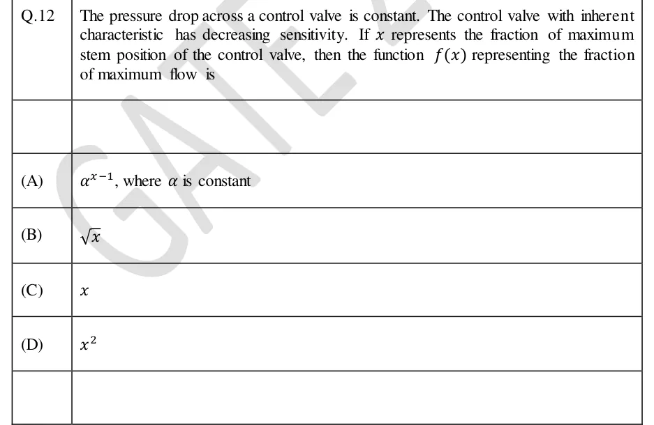
The pressure drop across a control valve is constant. The control valve with inherent characteristic has decreasing sensitivity. If $x$ represents the fraction of maximum stem position of the control valve, then the function $f (x)$ representing the fraction of maximum flow is

(A)
$α^{x - 1}$ , where $α$ is constant
(B)
$x$
(C)
$x$
(D)
$x^{2}$

Answer and solution

GATE 2024 IN Q.12: answer and solution

See the question in the paper

Tap to open full size

GATE 2024 IN Q.12: answer and solution

GATE 2022 IN Q.12

GATE 2022 · INQ.12 · 1 mark · MCQ

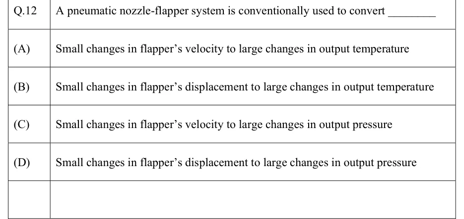
A pneumatic nozzle-flapper system is conventionally used to convert ________

(A)
Small changes in flapper's velocity to large changes in output temperature
(B)
Small changes in flapper's displacement to large changes in output temperature
(C)
Small changes in flapper's velocity to large changes in output pressure
(D)
Small changes in flapper's displacement to large changes in output pressure

Answer and solution

GATE 2022 IN Q.12: answer and solution

See the question in the paper

Tap to open full size

GATE 2022 IN Q.12: answer and solution

PRACTICE

7 questions to test yourself

PRACTICE 11 mark · MCQ

An equal-percentage control valve with rangeability 32 operates at constant pressure drop. At 80% of full stem travel, the flow through it, as a percentage of its maximum flow, is

(A)
80%
(B)
64%
(C)
50%
(D)
25%

Answer and solution

Answer: (C)

Equal-percentage law: $f = R^{x - 1}$ with $R = 32$ and $x = 0.8$ .
$f = 3 2^{- 0.2} = (2^{5})^{- 0.2} = 2^{- 1} = 0.5$ .
So the flow is 50% of maximum. (80% would be a linear valve; 25% is the equal-percentage flow at 60% travel.)

PRACTICE 22 marks · NAT

A unity negative-feedback system has open-loop transfer function $G (s) = \frac{20 e ^{- s T}}{s ( s + 3 )}$ , where $T \geq 0$ is a dead time in seconds. The closed loop is stable for $0 \leq T < T_{m a x}$ . The value of $T_{m a x}$ in seconds, rounded to three decimal places, is ______.

Answer and solution

Answer: $0.161$ (accepted range $\pm 0.002$ )

$∣ G (j ω) ∣ = \frac{20}{ω ω ^{2} + 9} = 1 \Rightarrow ω^{4} + 9 ω^{2} - 400 = 0 \Rightarrow ω^{2} = 16$ , so $ω_{g c} = 4$ rad/s, the only crossover (the delay does not change the magnitude).
Delay-free phase at 4 rad/s: $- 9 0^{\circ} - tan^{- 1} (4/3) = - 143.1 3^{\circ}$ , so $P M_{0} = 36.8 7^{\circ} = 0.6435$ rad.
A delay changes only the phase, so closed-loop poles can reach the imaginary axis only at a frequency where $∣ G (j ω) ∣ = 1$ , i.e. at $ω = 4$ rad/s. They get there when the extra lag $4 T$ uses up the whole phase margin. The loop is stable at $T = 0$ ( $P M_{0} > 0$ ), so it stays stable while $4 T < 0.6435$ .
$T_{m a x} = 0.6435/4 = 0.1609 \approx 0.161$ s.

PRACTICE 32 marks · NAT

In a unity negative-feedback loop with $G (s) = \frac{K e ^{- 0.5 s}}{s + 2}$ and $K > 0$ , the dead time is replaced by its first-order Pade approximation $e^{- s T} \approx \frac{1 - s T /2}{1 + s T /2}$ . The approximated closed loop is stable for $0 < K < K_{m a x}$ . The value of $K_{m a x}$ is ______.

Answer and solution

Answer: $6$

First-order Pade with $T = 0.5$ : $e^{- 0.5 s} \approx \frac{1 - 0.25 s}{1 + 0.25 s} = \frac{4 - s}{4 + s}$ .
Characteristic equation: $(s + 2) (s + 4) + K (4 - s) = 0 \Rightarrow s^{2} + (6 - K) s + (8 + 4 K) = 0$ .
A second-order polynomial is stable if and only if all its coefficients have the same sign; here both must be positive, so $K < 6$ (and $K > - 2$ ).
$K_{m a x} = 6$ . At $K = 6$ the equation is $s^{2} + 32 = 0$ , an oscillation at $32 = 5.66$ rad/s.
For comparison only: the exact limit comes from the phase crossover $tan^{- 1} (ω /2) + 0.5 ω = π$ , which gives $ω \approx 4.06$ rad/s and $K_{m a x} = ω^{2} + 4 \approx 4.52$ . The Pade value is optimistic, but the question asks for the Pade value, 6.

PRACTICE 41 mark · NAT

A variable-reluctance stepper motor has 24 stator teeth wound as 3 phases and 16 rotor teeth. It is driven in full-step mode, with one phase energised at a time, at 400 pulses per second. The shaft speed in rpm is ______.

Answer and solution

Answer: $500$

$β = \frac{36 0 ^{\circ}}{m N _{r}} = \frac{36 0 ^{\circ}}{3 \times 16} = 7. 5^{\circ}$ . Check: $\frac{24 - 16}{24 \times 16} \times 36 0^{\circ} = 7. 5^{\circ}$ .
$n = \frac{β f}{6} = \frac{7.5 \times 400}{6} = 500$ rpm. Equivalently, 48 steps per revolution, so $400/48$ rev/s $\times 60 = 500$ rpm.

PRACTICE 52 marks · MSQ

Which of the following statements is/are TRUE?

(A)
Adding a feedforward controller to an existing feedback loop leaves the closed-loop characteristic equation unchanged.
(B)
In cascade control, the secondary (inner) loop should have slower dynamics than the primary (outer) loop.
(C)
For safety on loss of instrument air, the fuel-gas valve to a furnace should be air-to-open (fail-closed).
(D)
A PLC with a 20 ms scan time, which reads its inputs once per scan, always detects an input pulse lasting 5 ms.

Answer and solution

Answer: (A), (C)

A is true: the feedforward path lies outside the loop, so $1 + G_{c} G_{v} G_{p} H = 0$ is unchanged.
B is false: the inner loop must be faster than the outer loop, or it cannot correct supply-side disturbances before they reach the primary variable.
C is true: an air-to-open valve fails closed, which shuts off fuel, the safe state.
D is false: inputs are read only during the input scan, so a 5 ms pulse can fall entirely between two input scans 20 ms apart and be missed.

PRACTICE 61 mark · NAT

A control valve has a flow coefficient $C_{v} = 20$ (US gal/min of water at a 1 psi drop, fully open). Fully open, it passes a liquid of specific gravity 0.81 with a pressure drop of 16 psi across the valve. The flow in US gal/min, rounded to one decimal place, is ______.

Answer and solution

Answer: $88.9$ (accepted range $\pm 0.2$ )

Liquid sizing equation with the valve fully open ( $f = 1$ ): $q = C_{v} Δ P / G$ .
$q = 20 16/0.81 = 20 \times \frac{4}{0.9} = 88.9$ US gal/min.
Note that $q \propto Δ P$ : at 4 psi the same valve would pass half this flow, not a quarter.

PRACTICE 71 mark · NAT

A unity negative-feedback loop has open-loop transfer function $G (s) = \frac{2 e ^{- s T}}{s}$ , where $T \geq 0$ is a dead time in seconds. The closed loop is stable for $0 \leq T < T_{m a x}$ . The value of $T_{m a x}$ in seconds, rounded to three decimal places, is ______.

Answer and solution

Answer: $0.785$ (accepted range $\pm 0.002$ )

$∣ G (j ω) ∣ = 2/ ω = 1$ at $ω_{g c} = 2$ rad/s, the only crossover.
Delay-free phase is $- 9 0^{\circ}$ at every frequency, so $P M_{0} = 9 0^{\circ} = π /2$ rad.
$T_{m a x} = P M_{0} / ω_{g c} = (π /2) /2 = π /4 = 0.785$ s. This agrees with the integrator-plus-dead-time condition $K T < π /2$ with $K = 2$ .

OFFICIAL GATE 2027 SYLLABUS WORDING

Copied from the GATE 2027 syllabus; see all 2027 syllabi.

GATE IN

time-delay systems. Actuators for control system: control valves, servo valves, servo motors, stepper motors; … cascade, feed forward, and ratio controllers …; basic concept of supervisory control, basics of distributed control system (DCS) and programmable logic controller (PLC)

Preparing in Kolkata? IAE Academy's course for GATE IN.