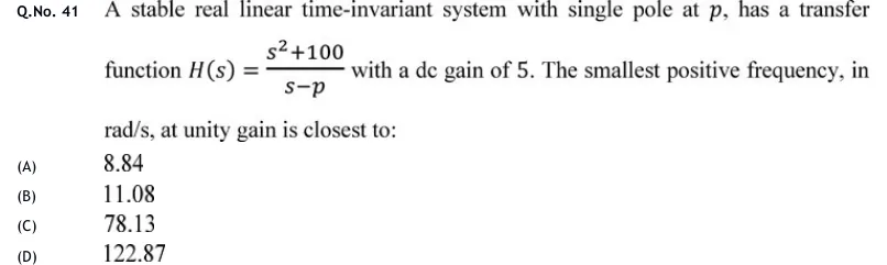
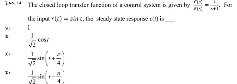
IAE Academy

GATE EC · EE · IN

Frequency response

Bode and polar plots, gain and phase margins

Frequency response describes what a stable linear system does to a sinusoid at each frequency: it scales the sinusoid by and shifts it by . From the open-loop , together with the number of open-loop poles in the right half plane, you can judge whether the closed loop is stable and how close it is to instability, using gain and phase margins, Bode asymptotes and polar plots. The core skills are: sketch or read a Bode plot, find where a polar plot starts, ends and crosses the axes, work out GM, PM, the largest allowable gain or delay, and link to resonant peak, bandwidth and phase margin.

27 previous-year questions · 26 solved · 6 practice questions

The sinusoidal transfer function

Drive a stable LTI system with . Once the transients die out, the output is a sinusoid of the same frequency. It is scaled by and shifted by . The function , which you get by putting , is the sinusoidal transfer function, and its behaviour as runs from to is the frequency response. A negative angle is a phase lag.

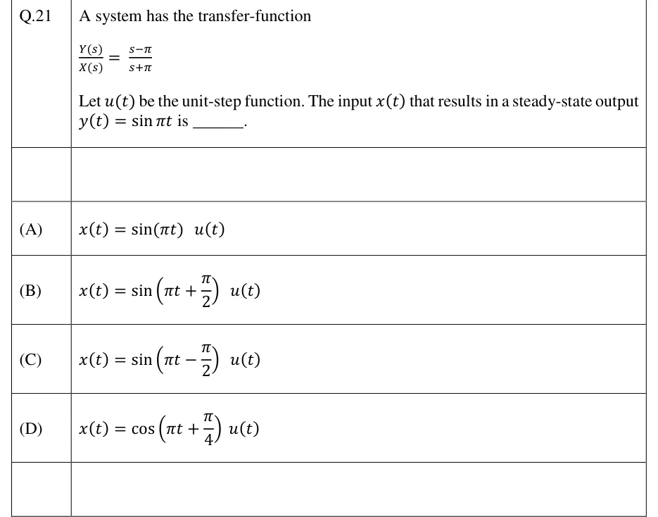
Quick check: take with input . Then , so and . The steady-state output is .

SINUSOIDAL STEADY-STATE RESPONSE

Valid only for a stable , after the transients decay. The frequency does not change, only the amplitude and phase.

Stability matters only for this physical reading. An unstable has no steady-state sinusoid, but you can still compute and plot , and that is exactly what the Nyquist criterion does with the open-loop function. Every margin in this topic is read from the open-loop of a negative-feedback loop, never from the closed-loop .

TIME-CONSTANT FORM: MAGNITUDES ADD IN DB, PHASES ADD

For and real poles and zeros in the left half plane (). A quadratic factor adds its own magnitude and phase terms (see the Bode table below). is the system type, the number of poles at the origin. This additive structure is why Bode plots are built factor by factor.

Frequency-domain specifications and their link to ζ

These specifications are read from the closed-loop response :

  • The resonant peak is the maximum value of .
  • The resonant frequency is the frequency where that maximum occurs.
  • The bandwidth is the frequency where falls to of its zero-frequency value , i.e. 3 dB below it.
  • The cut-off rate is the slope of the magnitude beyond .

Bandwidth measures speed. For the standard second-order system with fixed, is proportional to while rise time and settling time are proportional to , so doubling the bandwidth halves them. measures relative stability, as overshoot does in the time domain.

Take the standard second-order system . It is unity feedback around , so . Every specification follows from and . Throughout, write .

STANDARD SECOND-ORDER MAGNITUDE AND PHASE

, . The phase runs continuously from to , so pick the branch by whether is below or above 1.

VALUE AT THE NATURAL FREQUENCY

Holds for every . In dB the value is , which is 0 dB exactly when .

RESONANT FREQUENCY

Only for . In that range , where .

RESONANT PEAK

Only for . For there is no peak, falls monotonically, and at . depends on alone.

BANDWIDTH OF THE STANDARD SECOND-ORDER SYSTEM

The frequency where (−3 dB relative to ). Valid for every . exactly at and at .

BANDWIDTH OF A FIRST-ORDER SYSTEM

The bandwidth equals the corner frequency. A smaller time constant gives a wider bandwidth and a faster response.

PHASE MARGIN OF THE STANDARD SECOND-ORDER LOOP

For open loop with unity negative feedback. GM is infinite because the phase never reaches . Rough approximation: PM in degrees for , off by at most about 3.5°. Use the exact formula when the options are close.

(ratio / dB)

PM

(%)

0.2

2.55 / 8.14 dB

0.959

1.51

22.6°

52.7

0.3

1.75 / 4.85 dB

0.906

1.45

33.3°

37.2

0.4

1.36 / 2.70 dB

0.825

1.37

43.1°

25.4

0.5

1.15 / 1.25 dB

0.707

1.27

51.8°

16.3

0.6

1.04 / 0.35 dB

0.529

1.15

59.2°

9.5

0.707

1 / 0 dB (peak just vanishes)

0 (peak at )

1.00

65.5°

4.3

1.0

no peak ( at )

—

0.644

76.3°

0

EXAM TIP

Do not mix the two families of quantities. , and belong to the closed-loop . , , GM and PM belong to the open-loop . For the standard second-order system, , and PM depend on only, while , and all scale with .

EXAM TIP

A resonant peak needs , but time-domain overshoot needs only . A system with overshoots by about 1.5% and still has no resonant peak.

Bode plots: building them factor by factor

A Bode plot is a pair of graphs against : magnitude in dB and phase in degrees. On log scales, products become sums, so you plot each factor on its own and add them. Always rewrite the transfer function in time-constant form first, so that every factor looks like and the constant in front is the time-constant (Bode) gain . For a type-0 system this is the DC gain.

DECIBELS, DECADES AND SLOPES

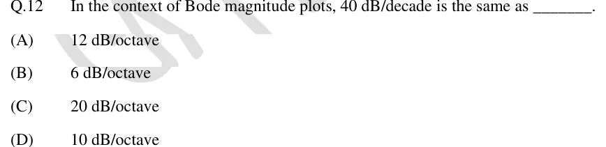
is the slope in dB/decade, and the relation holds along one straight segment. A decade is a factor of 10 and an octave a factor of 2, so 20 dB/decade 6.02 dB/octave.

Factor

Magnitude asymptote

Phase

Note

flat at

adds

(poles at origin)

straight line, dB/dec, through 0 dB at

(constant)

sets the low-frequency slope

(zeros at origin)

dB/dec through 0 dB at

low-frequency slope is positive

, simple pole

0 dB up to , then dB/dec

, at

exact value dB at

, LHP zero

0 dB up to , then dB/dec

, at

exact value dB at

0 dB up to , then dB/dec

, at

exact value at ; peak if

0 dB up to , then dB/dec

, at

exact value at ; dip if

, time delay

0 dB at every frequency

rad, grows without bound

changes phase only

SIMPLE-POLE EXACT VALUES NEAR THE CORNER Ω_C = 1/T

The errors are measured from the straight-line asymptote. The usual straight-line phase approximation (0° at , −45°/decade, −90° at ) is never off by more than 5.7°. For a zero, flip every sign.

LOW-FREQUENCY ASYMPTOTE AND ITS 0 DB CROSSING

must be the time-constant-form gain. The line (extended if necessary) reads at . Type 0: the plot starts flat at .

STATIC ERROR CONSTANTS FROM THE LOW-FREQUENCY ASYMPTOTE

For unity feedback, where , and . is the time-constant gain, is the flat low-frequency level in dB (type 0), and is where the low-frequency line, extended if needed, crosses 0 dB.

  1. Write in time-constant form and list the corner frequencies in ascending order.

  2. Draw the low-frequency asymptote with slope dB/decade through at . If lies beyond the first corner, extend the line to to locate it.

  3. Move right. At each corner, change the slope by for a simple pole, for a simple zero, for a quadratic pole pair and for a quadratic zero pair. A factor repeated times multiplies the change by .

  4. Check that the final slope is dB/decade, where is the number of poles and the number of zeros.

  5. If exact values are needed, correct the asymptote at each corner: dB for a simple pole, dB for a simple zero ( dB for a factor repeated times), for a quadratic pole pair and for a quadratic zero pair. Neighbouring corners add their own small errors, so this is exact only when corners are well separated.

  6. Phase: add the factor phases at a few chosen frequencies. For a minimum-phase function with it starts at and ends at .

EXAM TIP

The rule gives where the low-frequency line (extended) crosses 0 dB. If a corner lies below that frequency, the actual plot crosses 0 dB somewhere else, so walk along the segments instead.

EXAM TIP

A classic slip is using the pole-zero gain instead of the time-constant gain. For the time-constant gain is , not 100. The low-frequency line therefore reads dB at and, extended, crosses 0 dB at rad/s. The actual asymptotic plot does not cross there: it levels off at 20 dB between the zero corner at 2 rad/s and the pole corner at 10 rad/s, then falls at −20 dB/decade and crosses 0 dB at 100 rad/s.

Reading a transfer function; minimum phase, non-minimum phase and time delay

Reading a Bode plot means running the construction backwards. Slopes identify the factor types, the frequencies where the slope changes are the corners, and the low-frequency line gives the type and . A magnitude plot fixes the transfer function only if you are told it is minimum phase, because an RHP zero has exactly the same magnitude as its LHP mirror image.

  1. Initial slope dB/decade gives type . A slope of means a zero at the origin.

  2. Find from any point on the low-frequency line: . For type 0, is the flat starting level.

  3. A slope change of at is a zero . A change of is a pole . A change of is a double factor, or a quadratic if the plot shows a peak or dip; then follows from the height at .

  4. If the options are in pole-zero form, convert: , where the and are the corner frequencies (magnitudes of the poles and zeros).

WORKED EXAMPLE

The asymptotic Bode magnitude plot of a minimum-phase open-loop transfer function (unity negative feedback) has slope −40 dB/decade for rad/s, −20 dB/decade for rad/s and −40 dB/decade for rad/s. The asymptote reads 20 dB at rad/s. Find , the gain crossover frequency, the phase margin and the gain margin, and state whether the closed loop is stable.

Solution
  1. Initial slope −40 dB/decade, so the system is type 2. The +20 change at 2 is a zero and the −20 change at 10 is a pole . So .

  2. On the low-frequency line . At this is (20 dB), so .

  3. Pole-zero form: .

  4. Asymptotic crossover: for , , which is 2 (6.02 dB) at . For , at rad/s.

  5. Exact crossover: set and put . This gives , so and rad/s.

  6. Phase: . At 12.6 rad/s this is , so . The asymptotic 14.1 rad/s would give 27.2°, a fair estimate.

  7. For every , , so at all finite frequencies. There is no phase crossover, so GM .

  8. The open loop has no RHP poles and PM > 0, so the closed loop is stable. Check with Routh: has .

Answer: . rad/s (asymptotic estimate 14.1 rad/s), PM , GM . The closed loop is stable.

A minimum-phase transfer function has no poles or zeros in the right half s-plane and no time delay. For it, the magnitude plot fixes the phase uniquely, and the high-frequency slope dB/decade always comes with a final phase of (for ). A non-minimum-phase function has at least one RHP zero, or a delay. It has the same magnitude as its minimum-phase counterpart but more phase lag. Some texts also call a function with RHP poles non-minimum phase. For Bode reading, what matters is the RHP zero or the delay.

Property

Minimum phase

Non-minimum phase

Pole/zero location

all poles and zeros in the LHP, no delay

at least one RHP zero, or

Magnitude vs phase

phase fixed by the magnitude plot

same magnitude as the mirror-image LHP function, extra lag

High-frequency phase

, consistent with the slope dB/dec

more negative than ( extra per RHP zero); with a delay it goes to

Typical factor

: phase

: phase

RHP ZERO

Same magnitude as an LHP zero, but the phase is a lag. .

FIRST-ORDER ALL-PASS

. Magnitude is 0 dB everywhere and the phase goes from to , even though .

TIME DELAY

The magnitude plot is unchanged; the phase lag grows linearly with , which curves downward on a log-frequency axis. Remember 1 rad = 57.3°.

FIRST-ORDER PADÉ APPROXIMATION OF A DELAY

An all-pass, non-minimum-phase rational approximation. It is accurate at low frequencies ( small).

INTEGRATOR WITH DELAY

Negative feedback, , . The phase crossover comes from . Here crosses 1 only once, at , and the phase falls monotonically, so the margins decide stability. Equivalently PM must be positive.

EXAM TIP

Test for minimum phase on a given plot (with ): if the magnitude settles to dB/decade but the high-frequency phase ends below , or keeps falling without limit, there is an RHP zero or a delay. This test cannot detect an RHP pole, because at high frequency an RHP pole contributes , the same as an LHP pole.

EXAM TIP

A delay leaves the magnitude curve alone, so does not move, and it cuts PM by exactly radians. It also pulls lower, so when falls with frequency (the usual case) GM falls too. With a delay, the phase always reaches eventually, so GM is finite even for a first-order plant.

Polar plots

A polar plot is the locus of in the complex plane as goes from to . The distance from the origin is the magnitude, and the angle is measured from the positive real axis, counter-clockwise positive. When the phase lag grows with (the usual case), the locus therefore moves clockwise as increases. The Nyquist plot adds the mirror image for negative (and the detour arcs). To sketch a polar plot, find three things: the start (), the end () and the axis crossings.

START AND END POINTS

For a minimum-phase function with in time-constant form. The plot reaches the origin tangent to the axis at angle . If , it ends at the finite point equal to the ratio of the leading coefficients.

AXIS CROSSINGS

A crossing of the negative real axis happens at the phase crossover frequency . If the plot crosses at , then GM .

LOW-FREQUENCY ASYMPTOTE OF A TYPE-1 POLAR PLOT

The plot starts at infinity along −90°, running beside this vertical line. For the asymptote is .

(all , )

Start ()

End ()

Shape and crossings

semicircle in the 4th quadrant, centre , diameter ; at

crosses the negative imaginary axis at , value ; never crosses the negative real axis

crosses the negative real axis at , so GM is finite; with the crossing is at , so the closed loop is stable only for

the whole negative imaginary axis

vertical asymptote ; GM

crosses the negative real axis at , at

lies entirely in the 2nd quadrant; closed loop unstable for every

spirals into the origin

crosses the negative real axis infinitely many times

CONSTANT-M CIRCLES (UNITY FEEDBACK)

Unity negative feedback only. These are the loci in the plane where the closed-loop magnitude equals . For the circles lie left of , each encloses , and they shrink onto as . The resonant peak is the of the circle the polar plot is tangent to (the highest it reaches), and is the frequency at the point of tangency.

EXAM TIP

Multiplying by rotates every point of the plot by and scales it by . Each extra simple LHP pole adds to the final approach angle. This is how you get the start and end of any plot in the table without computing anything.

EXAM TIP

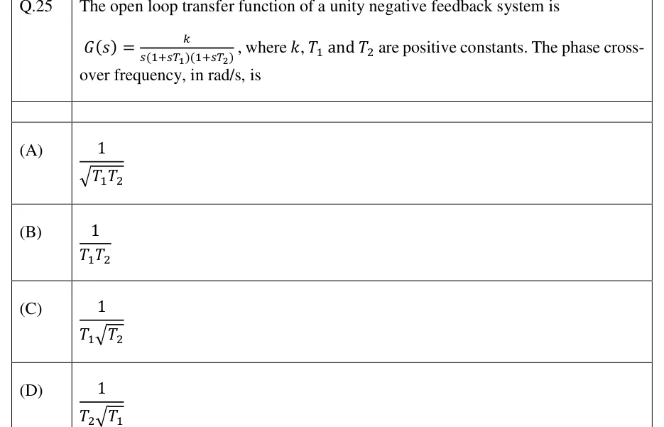
To find where a polar plot crosses the negative real axis, rationalise , set the imaginary part to zero and solve for , then substitute back. For two simple poles plus an integrator, you can skip the algebra: the crossing is at .

Gain margin and phase margin

Convention: negative feedback, open-loop , , and phase written as a lag (a negative angle such as ). The gain crossover frequency is where (0 dB). The phase crossover frequency is where . Gain margin is the factor by which the loop gain can be multiplied before the closed loop reaches the edge of instability. Phase margin is the extra phase lag at that would bring it to the same edge. Both measure the distance of the plot from the critical point .

CROSSOVER FREQUENCIES

Both are open-loop quantities, found on the Bode plot or on the polar plot (unit circle and negative real axis).

GAIN MARGIN

If the polar plot crosses the negative real axis at , then GM . A positive dB value means stable, in the standard case described below.

PHASE MARGIN

Use the phase as a negative angle: gives PM . On the polar plot, PM is the angle from the negative real axis to the point where the plot meets the unit circle.

LARGEST GAIN AND LARGEST DELAY

is the gain at which GM was computed. is the delay that uses up the whole phase margin; it assumes a single gain crossover, which a delay does not move.

TYPE-1, THIRD-ORDER LOOP

. Comes from for . It agrees with the Routh result for . In pole-zero form with : and .

  1. The margins alone decide stability when the open loop has no RHP poles, and and each cross 1 and only once (the usual minimum-phase case).

  2. Reading off a Bode plot: GM (dB) is how far the magnitude curve lies below 0 dB at , and PM is how far the phase curve lies above at .

  3. Stable: GM > 1 (GM > 0) and PM > 0, which is the same as .

  4. Marginally stable: GM = 1 (0 dB) and PM = 0, so . The closed loop oscillates steadily at that frequency.

  5. Unstable: GM < 1 (negative dB) and PM < 0, so .

  6. If the phase stays above at every finite frequency (for example any first-order loop, or with all ), there is no phase crossover and GM . A double integrator is different: its phase is exactly at every frequency, PM , and the closed loop is marginally stable. If at every frequency, there is no gain crossover and PM is taken as .

  7. For open-loop-unstable or conditionally stable loops, the margins can mislead, so apply the Nyquist criterion instead: . Here counts clockwise encirclements of by the plot of as traverses the Nyquist contour clockwise, is the number of open-loop RHP poles, and the closed loop is stable only if .

NYQUIST CRITERION (CLOCKWISE CONVENTION)

counts closed-loop RHP poles, open-loop RHP poles and clockwise encirclements of , with the Nyquist contour traversed clockwise. Texts that count counter-clockwise encirclements write .

WORKED EXAMPLE

For the loop with negative feedback, find the gain margin (in dB), the phase margin, the gain at which the closed loop becomes marginally stable, and the largest pure time delay that can be inserted before instability.

Solution
  1. Phase: . Setting it to needs , so and rad/s.

  2. .

  3. GM , i.e. dB. The gain can rise to . Check: . Routh on also needs , i.e. .

  4. Gain crossover: solve by trial. At the right side is , so rad/s (more precisely 2.454 rad/s).

  5. , so PM .

  6. PM rad, so s.

  7. , GM > 0 dB and PM > 0, consistent with a stable closed loop.

Answer: GM = 3 (9.54 dB), PM ≈ 25.4°, marginal gain K = 12, largest delay ≈ 0.18 s.

EXAM TIP

GM in dB is . If the polar plot cuts the negative real axis at , GM = +12.04 dB, not −12 dB.

EXAM TIP

Raising lifts the magnitude curve only. The phase curve and stay put, moves right, PM falls, and GM (dB) falls by of the factor. A delay acts on the other curve: magnitude and stay put, the phase curve drops, moves left, and PM falls by radians.

EXAM TIP

If a phase comes out as, say, (for example from a calculator's branch), convert it to the equivalent lag before using PM . Track the quadrant from the factor phases, not from a single of the ratio.

PREVIOUS-YEAR QUESTIONS

27 questions from the EC, EE and IN papers

Try each question first, then open the answer. One shows the official answer only. We placed each question under a topic ourselves; the exam paper does not label topics.

See these papers in full: GATE ECE 2025 · GATE ECE 2024 · GATE ECE 2023 · GATE ECE 2020 · GATE ECE 2018 · GATE EE 2026 · GATE EE 2024 · GATE EE 2023 · GATE EE 2022 · GATE EE 2020 · GATE IN 2026 · GATE IN 2024 · GATE IN 2023 · GATE IN 2022 · GATE IN 2020 · GATE IN 2018

GATE 2026 EE Q.29

GATE 2026 · EEQ.29 · 1 mark · MCQ

The asymptotic Bode magnitude plot of a system is shown.

[Figure]

Which one of the following options best represents the transfer function of the system?
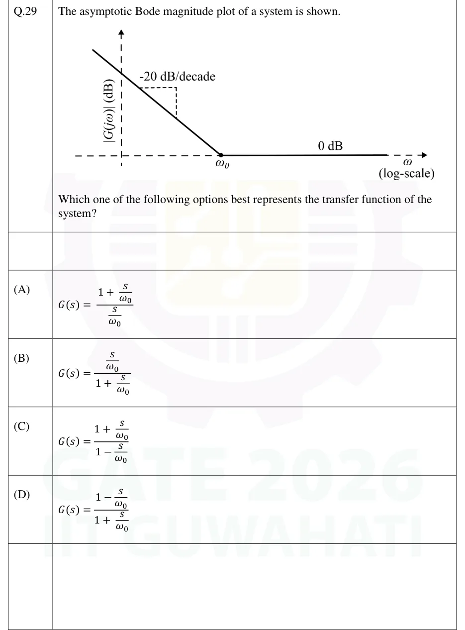
GATE 2026 EE question 29: Asymptotic Bode magnitude plot.Tap to open full size
Figure from the GATE 2026 EE paper. It is part of the question.
Figure description

Asymptotic Bode magnitude plot. Vertical axis: |G(j ω)| (dB), drawn as a dashed vertical line with an arrow. Horizontal axis: ω (log-scale), drawn as a dashed horizontal line at the 0 dB level with an arrow. The plot starts at the upper left (at frequencies below the vertical axis position, i.e. very low ω) as a straight line falling with slope labelled "-20 dB/decade" (a small dashed right-angle slope triangle drawn beside it). This falling line meets the 0 dB axis at a marked point (dot) labelled ω_0. From ω_0 onward the plot is a flat horizontal solid line labelled "0 dB" lying on the frequency axis, continuing to high frequencies. No other break points are shown.

  1. (A)

  2. (B)

  3. (C)

  4. (D)

Answer and solution
GATE 2026 EE Q.29: answer and solution

GATE 2025 EC Q.16

GATE 2025 · ECQ.16 · 1 mark · MCQ

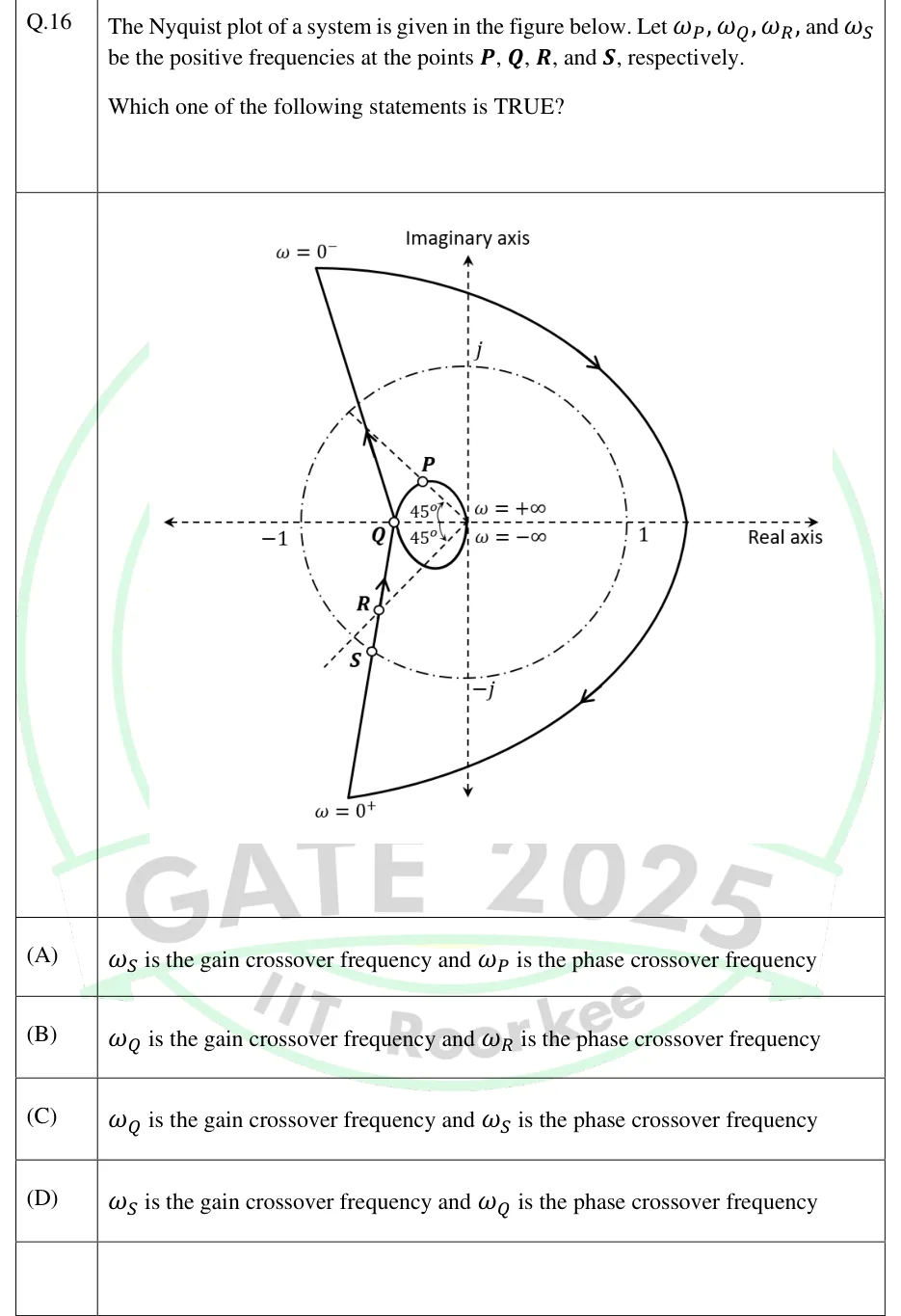
The Nyquist plot of a system is given in the figure below. Let , , , and be the positive frequencies at the points , , , and , respectively.

Which one of the following statements is TRUE?

GATE 2025 EC question 16: Nyquist plot in the complex plane.Tap to open full size
Figure from the GATE 2025 EC paper. It is part of the question.
Figure description

Nyquist plot in the complex plane. The real axis (labelled 'Real axis') and the imaginary axis (labelled 'Imaginary axis') are dashed. A dash-dot unit circle centred at the origin passes through the labelled points -1, 1, j and -j. Two dashed rays leave the origin into the left half-plane, 45° above and 45° below the negative real axis (each angle marked 45°), i.e. along ∠ 135° and ∠ -135°. The point labelled ω = 0^- is at the top left (about -0.95 + j1.6) and ω = 0^+ is at the bottom left (about -0.75 - j1.75). A large arc on the right joins them clockwise (arrows pointing clockwise) and crosses the positive real axis at about +1.4. From ω = 0^+ a nearly straight branch rises (arrow pointing upward). It first passes through point S, where it crosses the unit circle. It then passes through point R, where it crosses the -135° ray inside the unit circle, and reaches point Q on the negative real axis at about -0.45. S is not on the ray: the -135° ray meets the unit circle at an unlabelled point a little up and to the left of S, so S sits at an angle of roughly -125°. From Q a small loop continues. Its upper half passes through point P, where the 135° ray crosses it inside the unit circle, and ends at the origin, labelled ω = + ∞. Its lower half runs from the origin (labelled ω = - ∞) back to Q. From Q a second nearly straight branch, drawn roughly as the mirror image of the lower one, goes up and to the left to ω = 0^- (arrow pointing upward, away from Q).

  1. (A)

    is the gain crossover frequency and is the phase crossover frequency

  2. (B)

    is the gain crossover frequency and is the phase crossover frequency

  3. (C)

    is the gain crossover frequency and is the phase crossover frequency

  4. (D)

    is the gain crossover frequency and is the phase crossover frequency

Answer and solution
GATE 2025 EC Q.16: answer and solution

GATE 2024 EE Q.58

GATE 2024 · EEQ.58 · 2 marks · NAT

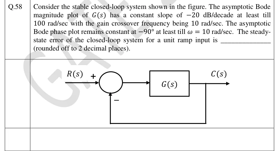
Consider the stable closed-loop system shown in the figure. The asymptotic Bode magnitude plot of has a constant slope of dB/decade at least till rad/sec with the gain crossover frequency being rad/sec. The asymptotic Bode phase plot remains constant at at least till rad/sec. The steady-state error of the closed-loop system for a unit ramp input is ________ (rounded off to 2 decimal places).

GATE 2024 EE question 58: Unity negative feedback loop.Tap to open full size
Figure from the GATE 2024 EE paper. It is part of the question.
Figure description

Unity negative feedback loop. Input R(s) enters a summing junction with a + sign; the output of the junction feeds a single forward block G(s) whose output is C(s). C(s) is taken back directly (gain 1) to the summing junction with a - sign. No other blocks.

Answer and solution
GATE 2024 EE Q.58: answer and solution

GATE 2024 EE Q.59

GATE 2024 · EEQ.59 · 2 marks · NAT

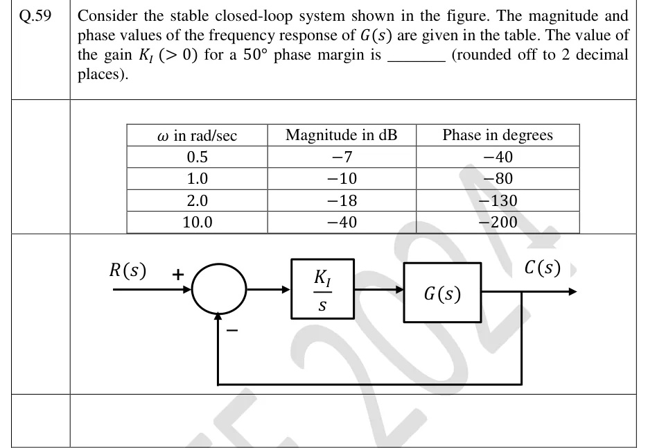
Consider the stable closed-loop system shown in the figure. The magnitude and phase values of the frequency response of are given in the table. The value of the gain for a phase margin is ________ (rounded off to 2 decimal places).

| in rad/sec | Magnitude in dB | Phase in degrees |
|---|---|---|
| 0.5 | | |
| 1.0 | | |
| 2.0 | | |
| 10.0 | | |

GATE 2024 EE question 59: Unity negative feedback loop.Tap to open full size
Figure from the GATE 2024 EE paper. It is part of the question.
Figure description

Unity negative feedback loop. R(s) enters a summing junction with a + sign; the feedback enters the same junction from below with a - sign. The junction output goes to a block (K_I)/(s), which feeds a block G(s) in cascade. The output of G(s) is C(s), and C(s) is fed back directly (unity gain, no block) to the negative input of the summing junction. The frequency-response table of G(s) is printed above the diagram.

Answer and solution
GATE 2024 EE Q.59: answer and solution

GATE 2024 IN Q.18

GATE 2024 · INQ.18 · 1 mark · MCQ

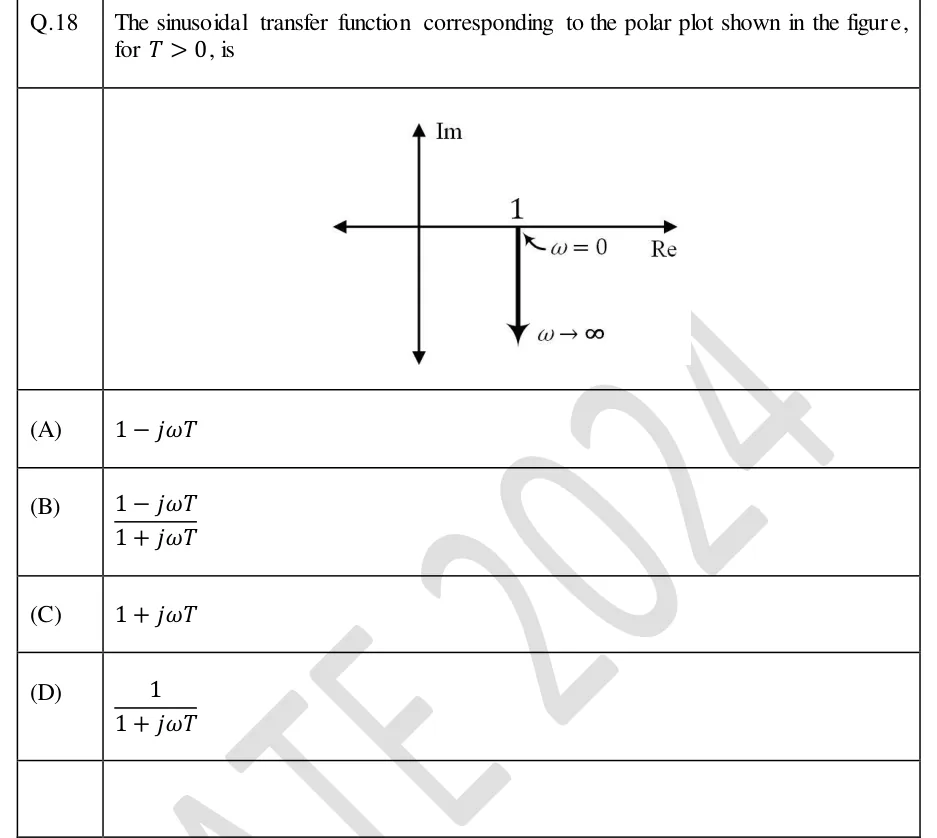
Q.18 The sinusoidal transfer function corresponding to the polar plot shown in the figure, for , is

GATE 2024 IN question 18: Polar plot on Re–Im axes (horizontal axis labelled Re, vertical axis labelled Im, both drawn with arrows at both ends).Tap to open full size
Figure from the GATE 2024 IN paper. It is part of the question.
Figure description

Polar plot on Re–Im axes (horizontal axis labelled Re, vertical axis labelled Im, both drawn with arrows at both ends). The point 1 is marked on the positive real axis, labelled with an arrow as ω = 0. From this point a straight vertical line is drawn downward (parallel to the negative imaginary axis, at constant real part 1), ending in an arrowhead labelled ω → ∞. So the locus starts at 1 + j0 and runs straight down along Re = 1 towards -j ∞.

  1. (A)

  2. (B)

  3. (C)

  4. (D)

Answer and solution
GATE 2024 IN Q.18: answer and solution

GATE 2023 EC Q.57

GATE 2023 · ECQ.57 · 2 marks · NAT

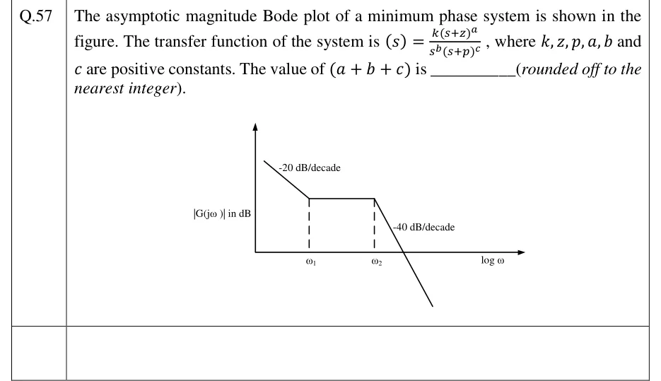
The asymptotic magnitude Bode plot of a minimum phase system is shown in the figure. The transfer function of the system is , where and are positive constants. The value of is ________ (rounded off to the nearest integer).

GATE 2023 EC question 57: Asymptotic Bode magnitude plot.Tap to open full size
Figure from the GATE 2023 EC paper. It is part of the question.
Figure description

Asymptotic Bode magnitude plot. Vertical axis labelled |G(jω)| in dB; horizontal axis labelled log ω. The plot starts at low frequency as a straight line falling with slope labelled -20 dB/decade until frequency ω1 (dashed vertical line to the axis). From ω1 to ω2 (second dashed vertical line) the plot is a horizontal line (0 dB/decade) at a positive dB level. After ω2 the plot falls steeply with slope labelled -40 dB/decade, crossing the log ω axis (0 dB) and continuing below it. No numerical values are given for ω1, ω2 or the dB levels.

Answer and solution
GATE 2023 EC Q.57: answer and solution

GATE 2023 EE Q.36

GATE 2023 · EEQ.36 · 2 marks · MCQ

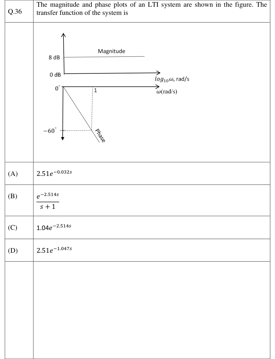
The magnitude and phase plots of an LTI system are shown in the figure. The transfer function of the system is

GATE 2023 EE question 36: Two plots stacked vertically.Tap to open full size
Figure from the GATE 2023 EE paper. It is part of the question.
Figure description

Two plots stacked vertically. Top (Magnitude): vertical axis marked 0 dB and 8 dB; horizontal axis labelled log_10 ω, rad/s. The magnitude is a flat horizontal line at 8 dB for all frequencies. Bottom (Phase): horizontal axis labelled ω (rad/s) on a linear scale, starting at 0 degrees at the origin; vertical axis pointing downward, marked 0 degrees and -60 degrees. The phase is a straight line starting at 0 degrees at ω = 0 and falling linearly; dashed lines show it passes through -60 degrees at ω = 1 rad/s. The line is labelled 'Phase'.

  1. (A)

  2. (B)

  3. (C)

  4. (D)

Answer and solution
GATE 2023 EE Q.36: answer and solution

GATE 2023 IN Q.43

GATE 2023 · INQ.43 · 2 marks · MCQ

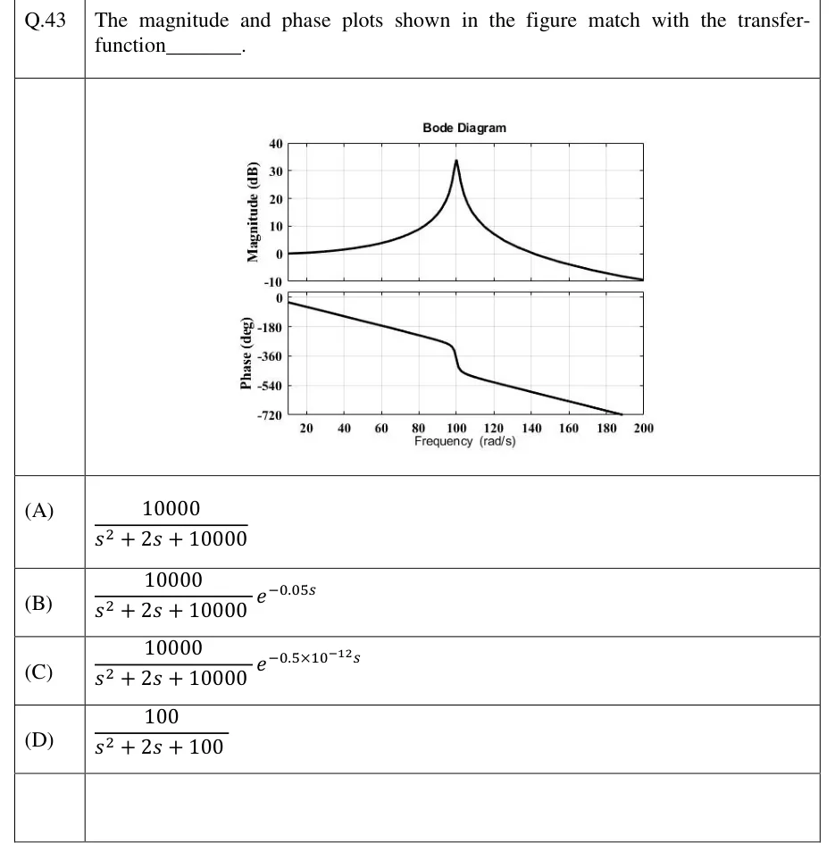
The magnitude and phase plots shown in the figure match with the transfer-function ________.

GATE 2023 IN question 43: A plot titled 'Bode Diagram' with two stacked panels that share a LINEAR frequency axis labelled 'Frequency (rad/s)'.Tap to open full size
Figure from the GATE 2023 IN paper. It is part of the question.
Figure description

A plot titled 'Bode Diagram' with two stacked panels that share a LINEAR frequency axis labelled 'Frequency (rad/s)'. The axis runs from about 10 rad/s at the left edge to 200 rad/s, with ticks at 20, 40, 60, 80, 100, 120, 140, 160, 180 and 200. Top panel: 'Magnitude (dB)', axis from -10 to 40 (ticks -10, 0, 10, 20, 30, 40). The curve starts at 0 dB at the left edge, rises slowly and then steeply to a sharp resonant peak of about 33 to 34 dB at 100 rad/s, then falls, crossing 0 dB near 140 rad/s and ending just above -10 dB at 200 rad/s. Bottom panel: 'Phase (deg)', axis from -720 to 0 (ticks 0, -180, -360, -540, -720). The phase is about -30 deg at the left edge (about 10 rad/s). It falls along a straight line (linear in omega), crosses -180 deg a little past 60 rad/s and reaches about -300 deg just below 100 rad/s. Around 100 rad/s it drops steeply by roughly 150 to 180 deg to about -450 deg. It then keeps falling along a straight line of the same slope and leaves the bottom of the axes at -720 deg at about 189 rad/s.

  1. (A)

  2. (B)

  3. (C)

  4. (D)

Answer and solution
GATE 2023 IN Q.43: answer and solution

GATE 2022 EE Q.17

GATE 2022 · EEQ.17 · 1 mark · MCQ

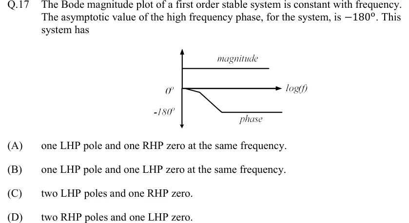
The Bode magnitude plot of a first order stable system is constant with frequency. The asymptotic value of the high frequency phase, for the system, is . This system has

GATE 2022 EE question 17: Sketch of a Bode plot.Tap to open full size
Figure from the GATE 2022 EE paper. It is part of the question.
Figure description

Sketch of a Bode plot. A vertical axis with arrowheads at both ends carries two labels on its left, 0° (level with the horizontal axis) and -180° (below it). The horizontal axis is labelled log (f). A curve labelled 'magnitude' is a flat horizontal line drawn above the horizontal axis, constant at every frequency. A curve labelled 'phase' starts at 0° on the vertical axis, falls gently for a short stretch, then falls more steeply in a straight line, and then levels off as a flat asymptote at -180° at high frequency.

  1. (A)

    one LHP pole and one RHP zero at the same frequency.

  2. (B)

    one LHP pole and one LHP zero at the same frequency.

  3. (C)

    two LHP poles and one RHP zero.

  4. (D)

    two RHP poles and one LHP zero.

Answer and solution
GATE 2022 EE Q.17: answer and solution

GATE 2022 EE Q.37

GATE 2022 · EEQ.37 · 2 marks · MCQ

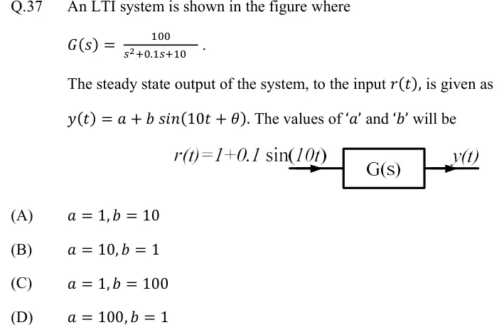
An LTI system is shown in the figure where

The steady state output of the system, to the input , is given as . The values of '' and '' will be

GATE 2022 EE question 37: A single block labelled G(s).Tap to open full size
Figure from the GATE 2022 EE paper. It is part of the question.
Figure description

A single block labelled G(s). An input arrow enters from the left labelled r(t) = 1 + 0.1 sin(10t); an output arrow leaves on the right labelled y(t). No feedback path, no summing junction: this is an open-loop cascade of input into G(s).

  1. (A)

  2. (B)

  3. (C)

  4. (D)

Official answer

Official answer: ASource: Official answer key, GATE 2022 EE (IIT Kharagpur)

A NOTE ON THIS QUESTION

As printed, none of the four options is correct. The paper gives and . The DC term gives . At : , so and . No option has with . The official key is (A), and , which is what the same working gives if the constant term of the denominator is instead of : then and , so and . The printed question appears to contain a misprint. We show the official answer, and we do not publish a worked solution that the printed numbers do not lead to.

GATE 2022 EE Q.37: official answer

GATE 2022 IN Q.43

GATE 2022 · INQ.43 · 2 marks · MCQ

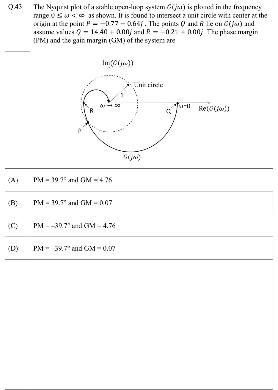
The Nyquist plot of a stable open-loop system is plotted in the frequency range as shown. It is found to intersect a unit circle with center at the origin at the point . The points and lie on and assume values and . The phase margin (PM) and the gain margin (GM) of the system are ________

GATE 2022 IN question 43: Nyquist plot on axes Re(G(jω)) (horizontal, arrow to the right) and Im(G(jω)) (vertical, arrow upward).Tap to open full size
Figure from the GATE 2022 IN paper. It is part of the question.
Figure description

Nyquist plot on axes Re(G(jω)) (horizontal, arrow to the right) and Im(G(jω)) (vertical, arrow upward). A dashed unit circle is centred at the origin. A radius arrow from the origin to the upper right is labelled 1, and the label 'Unit circle' has an arrow pointing to the circle. The solid curve, labelled G(jω) under its lower arc, starts at the point labelled Q on the positive real axis, well outside the circle, where it is marked ω=0. From Q it runs clockwise: down through the fourth quadrant in a large arc beneath the origin, then into the third quadrant, where it meets the dashed circle at the point labelled P (lower left). It then rises and crosses the negative real axis at the point labelled R, drawn just inside the left edge of the circle. After that it curls up into the second quadrant in a small loop above the axis and comes down into the origin from above, where it is marked ω → ∞. Only the letters P, Q and R are printed on the figure; their numerical values are given in the stem. The point −1 is not marked, and the figure is not to scale (R = −0.21 is drawn close to the circle's edge).

  1. (A)

    and

  2. (B)

    and

  3. (C)

    and

  4. (D)

    and

Answer and solution
GATE 2022 IN Q.43: answer and solution

GATE 2018 EC Q.42

GATE 2018 · ECQ.42 · 2 marks · NAT

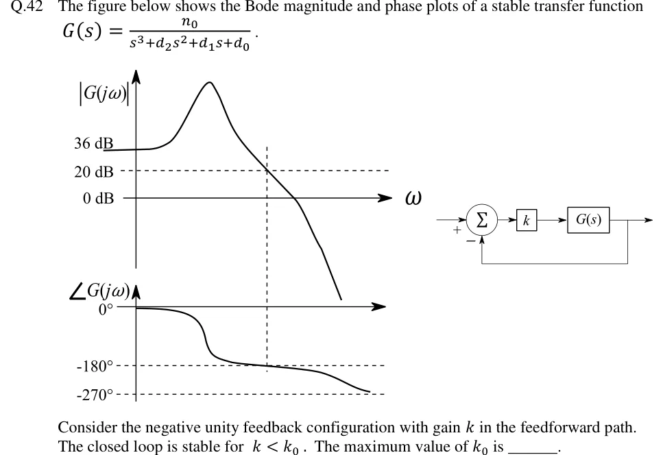
The figure below shows the Bode magnitude and phase plots of a stable transfer function .

Consider the negative unity feedback configuration with gain in the feedforward path. The closed loop is stable for . The maximum value of is ______.

GATE 2018 EC question 42: Left: Bode plots sharing a common frequency axis.Tap to open full size
Figure from the GATE 2018 EC paper. It is part of the question.
Figure description

Left: Bode plots sharing a common frequency axis. Magnitude plot: vertical axis |G(j ω)| with marked levels 36 dB, 20 dB (dashed horizontal line) and 0 dB (the ω axis). The curve starts flat at 36 dB at low frequency, rises to a sharp resonant peak, then falls, crossing the 20 dB dashed line at a frequency marked by a vertical dashed line, then crosses 0 dB, then drops steeply. Phase plot: vertical axis ∠ G(j ω) with marked levels 0°, -180° (dashed) and -270° (dashed). The phase starts at 0°, drops sharply near the resonant frequency to just above -180°, then decreases slowly and crosses -180° exactly at the same vertical dashed frequency where the magnitude is 20 dB, then continues down towards -270° at high frequency. Right: block diagram — reference enters a summing junction with sign +, the junction output goes to a gain block k, then to block G(s), whose output is the system output; the output is fed back with unity gain to the summing junction with sign −.

Answer and solution
GATE 2018 EC Q.42: answer and solution

GATE 2018 IN Q.13

GATE 2018 · INQ.13 · 1 mark · MCQ

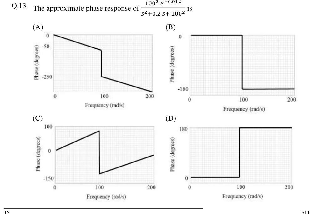
The approximate phase response of is

GATE 2018 IN question 13: All four options are phase plots.Tap to open full size
Figure from the GATE 2018 IN paper. It is part of the question.
Figure description

All four options are phase plots. In each one the horizontal axis is Frequency (rad/s) running from 0 to 200, with a tick label at 100, and the vertical axis is Phase (degrees). (A) Axis labels at 0, -50 and -250. The labels are not evenly spaced: the gap from 0 to -50 is about a third of the gap from -50 to -250. So the plot is a sketch, not a scaled graph. A straight line falls from (0, 0) to a corner just below 100 rad/s, a little below the -50 label (roughly -70 degrees on the printed labels). There the phase drops vertically to the level of the -250 label. It then falls in a straight line with the same slope as the first segment, reaching the bottom edge of the plot at 200 rad/s (roughly -345 degrees on the printed labels). (B) Axis labels at 0 and -180. The phase is flat at 0 from 0 to 100 rad/s, steps down vertically to -180 at 100 rad/s, and stays flat at -180 out to 200 rad/s. (C) Axis labels at 100, 0 and -150. A straight line rises from (0, 0) to about +80 degrees at 100 rad/s. It drops vertically to about -120 degrees (above the -150 label), then rises in a straight line to about -20 degrees at 200 rad/s. (D) Axis labels at 0 and 180. The phase is flat at 0 from 0 to 100 rad/s, steps up vertically to +180 at 100 rad/s, and stays flat at +180 out to 200 rad/s.

  1. (A)

    Figure: phase falls in a straight line from 0 to a little below the -50 label just before 100 rad/s, drops vertically to the -250 label, then keeps falling with the same slope to the bottom of the plot at 200 rad/s.

  2. (B)

    Figure: phase is flat at 0 up to 100 rad/s, steps down to -180 degrees and stays flat there out to 200 rad/s.

  3. (C)

    Figure: phase rises linearly from 0 to about +80 degrees at 100 rad/s, drops vertically to about -120 degrees, then rises linearly to about -20 degrees at 200 rad/s.

  4. (D)

    Figure: phase is flat at 0 up to 100 rad/s, steps up to +180 degrees and stays flat there out to 200 rad/s.

Answer and solution
GATE 2018 IN Q.13: answer and solution

PRACTICE

6 questions to test yourself

PRACTICE 12 marks · MCQ

The asymptotic Bode magnitude plot of a minimum-phase transfer function has slope −20 dB/decade for rad/s, 0 dB/decade for rad/s and −20 dB/decade for rad/s. The flat segment lies at 20 dB. Which option gives and the gain crossover frequency read from the asymptotic plot?

  1. (A)

    , rad/s

  2. (B)

    , rad/s

  3. (C)

    , rad/s

  4. (D)

    , rad/s

Answer and solution

Answer: (A)

  1. Initial slope −20 dB/decade means type 1. The +20 change at 1 rad/s is a zero and the −20 change at 5 rad/s is a pole .

  2. The low-frequency line meets the flat 20 dB segment at , so .

  3. .

  4. For , , which equals 1 at rad/s. Equivalently, the line falls 20 dB in one decade from 20 dB at 5 rad/s, reaching 0 dB at 50 rad/s. (The exact crossover is 49.8 rad/s.)

PRACTICE 22 marks · NAT

A negative-feedback loop has . Find the gain margin in dB, correct to two decimal places.

Answer and solution

Answer: (accepted range )

  1. Phase: . For you need , so rad/s.

  2. .

  3. GM , so GM dB.

  4. Check with Routh: is stable for , and .

PRACTICE 31 mark · NAT

A unity-feedback system has closed-loop transfer function . Find the resonant peak of as a ratio (not in dB), correct to two decimal places.

Answer and solution

Answer: (accepted range )

  1. Compare with : rad/s and , so .

  2. , so a resonant peak exists.

  3. .

  4. It occurs at rad/s.

PRACTICE 41 mark · MCQ

Consider and . Which one of the following statements is correct?

  1. (A)

    for all , and as

  2. (B)

    for all

  3. (C)

    as

  4. (D)

    at high frequencies

Answer and solution

Answer: (A)

  1. , so the magnitudes are identical at every . This rules out D.

  2. , which goes to as . This rules out C.

  3. , which goes to . The phases differ, which rules out B. is non-minimum phase because of its RHP zero at .

  4. So A is correct.

PRACTICE 52 marks · MSQ

A unity negative-feedback system has open-loop transfer function . Which of the following statements is/are correct?

  1. (A)

    The polar plot of starts at infinite magnitude along and reaches the origin tangent to the negative real axis (angle ).

  2. (B)

    The gain margin is infinite.

  3. (C)

    As , the polar plot approaches the vertical asymptote .

  4. (D)

    Inserting a pure time delay of 0.1 s in the loop makes the closed loop unstable.

Answer and solution

Answer: (A), (B), (C)

  1. A: the system is type 1, so it starts at . , so it ends at . Correct.

  2. B: stays above at every finite , so there is no phase crossover and GM . Correct.

  3. C: the type-1 asymptote is . Correct.

  4. D: gives , i.e. with . So and rad/s.

  5. , so PM rad and s.

  6. A 0.1 s delay removes only rad , leaving PM . The magnitude still crosses 1 only once and the phase still falls monotonically, so the system stays stable and D is wrong.

PRACTICE 61 mark · NAT

A unity negative-feedback loop has open-loop transfer function with . Find the largest value of for which the closed loop is stable, correct to two decimal places.

Answer and solution

Answer: (accepted range )

  1. The magnitude is , unaffected by the delay. It falls monotonically and crosses 1 once, at .

  2. The phase is , which falls monotonically. It reaches when , so rad/s.

  3. , so GM . The open loop has no RHP poles, so the closed loop is stable while GM > 1, i.e. .

  4. Cross-check with PM: , which is positive only for .

OFFICIAL GATE 2027 SYLLABUS WORDING

Copied from the GATE 2027 syllabus; see all 2027 syllabi.

GATE EC

Frequency response; … Bode … plots

GATE EE

Bode plots

GATE IN

Bode plot, phase and gain margins

Preparing in Kolkata? IAE Academy's course for GATE ECE, GATE EE or GATE IN.