IAE Academy

GATE EC · EE · IN

Time response and steady-state error

Time response is how a control system's output moves after a standard test input is applied. It has a transient part and a steady-state part. The closed-loop poles fix how fast the transient decays and oscillates. The steady-state part is fixed by the input and by the closed loop's behaviour at DC, which for unity feedback comes down to the type and gain of the open-loop transfer function. There are two core skills. The first is reading the damping ratio, natural frequency and time-domain specifications off a transfer function. The second is computing steady-state error from the system type and error constants, once you have checked that the closed loop is stable.

22 previous-year questions · 22 solved · 6 practice questions

Test inputs and the two parts of a response

After an input is applied, the output of a stable LTI system has two parts. The transient part dies out. Its modes (decay rates and oscillation frequencies) are set by the closed-loop poles, and the zeros also affect how much of each mode appears. The steady-state part is what is left as . The gap between it and the input is the steady-state error. That depends on the input and on how the closed-loop behaves near . For unity feedback, this comes down to how the open-loop behaves near .

Conventions used throughout these notes: negative feedback, zero initial conditions, inputs applied at , and error unless a question defines it another way.

Input

for

What it tests

Unit impulse

Natural response. The impulse response is the inverse Laplace transform of

Step of size

Response to a sudden change. All the transient specifications are defined on it

Ramp of slope

Following a constant velocity

Parabolic

Following a constant acceleration

EXAM TIP

With zero initial conditions, the impulse response is the time derivative of the step response, and the step response is the derivative of the ramp response. If you know one of them, differentiate or integrate to get the others.

EXAM TIP

The parabolic input is defined as . So an input has and . If you read it as , every parabolic error you compute comes out half the true value.

First-order systems and the time constant

A first-order system has one real pole. In time-constant form with , the pole is at , is the DC gain , and is the time constant. Without a zero, its step response never overshoots. The only things that matter are how fast it is () and where it ends up ().

FIRST-ORDER UNIT-STEP RESPONSE

For a unit step into . At the output has made 63.2% of its final change, and its initial slope is .

FIRST-ORDER SPECIFICATIONS

The exact settling values are and time constants. A first-order system without a zero has no peak time and no overshoot.

FIRST-ORDER UNIT-RAMP RESPONSE

For , which has unity DC gain. After the transient, the output runs parallel to the input but seconds behind it, so the steady-state error to a unit ramp is . This is the same as a unity-feedback loop with , whose .

CLOSING A UNITY LOOP AROUND A FIRST-ORDER PLANT

Unity negative feedback, with and . Feedback moves the pole from to , so the closed loop is faster than the plant. Its DC gain is less than 1. That gives a steady-state unit-step error of , the same as with .

EXAM TIP

Read only after putting the transfer function in time-constant form. For example, , so s and the DC gain is 2.5. Put another way, for a stable real pole at (). For a feedback system, use the closed-loop pole, not the open-loop one.

Second-order systems: damping ratio, natural frequency and pole location

A second-order system without zeros can be matched to one standard form. Write its denominator with a leading coefficient of 1 and check that the constant term is positive, then compare coefficients. Once matched, two numbers describe it completely. The damping ratio sets the shape of the response, and the undamped natural frequency sets its speed.

STANDARD SECOND-ORDER FORM

Unity DC gain. If the numerator is some other constant, and still come from the denominator. Only the final value changes.

UNDERDAMPED POLE LOCATION

Holds for . Here is the decay rate, is the damped frequency, and is the angle of the pole measured from the negative real axis.

Damping ratio

Name

Closed-loop poles

Unit-step response

Undamped

, on the imaginary axis

. Oscillates forever (marginally stable)

Underdamped

Complex conjugate pair in the left half plane

Oscillation that decays, with overshoot

Critically damped

Repeated real pole at

. For a given , the fastest response that does not overshoot

Overdamped

Two distinct real poles at

No overshoot. Slower than critical damping for the same

Negatively damped

Right half plane

Grows without limit. Unstable

UNDERDAMPED UNIT-STEP RESPONSE

For in the standard form. The oscillation stays inside the envelope . The settling-time formula is based on this envelope.

UNDERDAMPED UNIT-IMPULSE RESPONSE

The derivative of the step response above, for . It starts at zero and decays at the same envelope rate, .

OVERDAMPED UNIT-STEP RESPONSE

For : two distinct real poles at and , with . Note that and . When is much larger than , the term dies out quickly and .

UNITY FEEDBACK AROUND A TYPE-1 SECOND-ORDER PLANT

Unity negative feedback, with and . The loop is critically damped at and underdamped for . Raising raises and lowers . The real part of the poles, , stays fixed as long as .

EXAM TIP

What follows from the last result: for in the underdamped range (), increasing increases overshoot and shortens both rise time and peak time. The approximate 2% settling time, , does not change with . The exact settling time does change. The envelope amplitude depends on , and the response enters the band at a different peak. With , the exact value is about 1.05 s at and about 0.83 s at , while s for both.

EXAM TIP

An overdamped system has two real poles, at and , so it has two time constants, and . If one pole is several times further from the origin than the other, the response is close to a first-order response set by the slower pole (the one nearer the origin), with the DC gain kept.

Time-domain specifications of the underdamped step response

  1. Delay time : the time taken to reach 50% of the final value.

  2. Rise time : from 0 to 100% of the final value for an underdamped system. For first-order and overdamped systems it is measured from 10 to 90%, because they never reach 100% in finite time. The 10 to 90% definition is also used for underdamped systems, so follow whatever the question states. The formula below gives the 0 to 100% value.

  3. Peak time : the time to the first maximum.

  4. Peak overshoot , usually quoted in percent.

  5. Settling time : the time after which the response stays within ±2% (or ±5%) of the final value.

All of these refer to a unit-step input with zero initial conditions. The formulas below assume the standard form with no zeros and . Overshoot is measured relative to the final value, so a DC gain other than 1 does not change .

RISE TIME (0 TO 100%)

Underdamped systems only. must be in radians.

PEAK TIME

Half of the damped period . It depends only on the imaginary part of the poles.

PEAK OVERSHOOT

Valid for , and depends only on . For the step response has no overshoot.

DAMPING RATIO FROM OVERSHOOT

Enter as a fraction (0.163, not 16.3). This is what you use in design questions that specify the overshoot.

SETTLING TIME

Envelope approximations for . They give the time it takes to fall to about 2% () or 5% (), and is the time constant of the envelope. They are not the exact time at which the response enters the band for good. For the worked example below, the 2% formula gives 1.33 s and the exact value is about 1.19 s. Use these formulas unless the question gives a different rule.

DELAY TIME (APPROXIMATE)

An empirical approximation for , within about 5% of the exact value over that range.

SUCCESSIVE PEAKS AND LOGARITHMIC DECREMENT

For . are overshoots on the same side of the final value, one damped period apart. More generally, the -th extremum of the unit-step response (at ) differs from the final value by times the final value, falling alternately above and below it.

OSCILLATIONS BEFORE SETTLING

The number of damped cycles completed within the settling time, using the approximation . With the 5% rule, , it is .

Damping ratio

Peak overshoot

0.2

52.7%

0.4

25.4%

0.5

16.3%

0.6

9.5%

0.707 ()

4.3% ()

0.8

1.5%

1 or more

0 (no overshoot)

  1. Poles on a horizontal line (same ) have the same peak time, .

  2. Poles on a vertical line (same ) have the same approximate settling time, .

  3. Poles on a radial line from the origin (same , so same ) have the same overshoot.

  4. Poles on a circle centred at the origin have the same .

  5. Moving the poles further left shortens . Moving them further from the real axis shortens and raises the oscillation frequency.

WORKED EXAMPLE

A unity negative-feedback system has . For a unit-step input, find , , the peak overshoot, the peak time, the rise time and the 2% settling time. Also find the steady-state error for a unit-ramp input.

Solution
  1. Closed loop: .

  2. Compare with the standard form: rad/s, and .

  3. and rad/s, so the poles are at . Both are in the left half plane, so the loop is stable and the final value theorem can be used for the error.

  4. , which is 9.48%.

  5. s.

  6. rad, so s.

  7. s. With the 5% band it would be s. These are the formula values. The exact response settles into the 2% band at about 1.19 s and into the 5% band at about 1.05 s.

  8. has one pole at the origin, so the system is type 1. , which gives for a unit ramp.

Answer: , rad/s, , s, s, s by the rule, unit-ramp .

EXAM TIP

If stays fixed, raising lowers overshoot but lengthens both rise time and peak time, while the approximate settling time gets shorter. You cannot get a faster rise and less overshoot just by changing damping.

EXAM TIP

Common slips: using degrees for in ( rad, not 53.13°); using instead of in ; putting into the formula in percent; and applying these formulas to a system that has a zero or a third pole close to the dominant pair.

Extra poles and zeros, and dominant poles

Real systems are rarely pure second-order. Before judging the effect of an added pole or zero, check where it was added. Adding it to the closed-loop transfer function changes the response directly. Adding it to the open-loop moves the closed-loop poles, as the root locus shows. A zero added to the forward path also appears as a zero of .

EFFECT OF A CLOSED-LOOP ZERO

The zero is at with , and the DC gain is unchanged. The derivative term is positive while the output rises, so the response rises faster and overshoots more (or starts to overshoot). The effect fades as grows.

  1. Closed-loop LHP zero: and get shorter and gets larger. The nearer the zero is to the origin, the stronger the effect.

  2. Closed-loop LHP pole: the response gets slower ( grows) and overshoot is usually smaller. A pole far to the left has almost no effect.

  3. Closed-loop RHP zero (non-minimum phase): with one real RHP zero (more generally, an odd number of them), the step response first moves the wrong way (undershoot) and only then heads to its final value.

  4. Open-loop pole added to : the root locus is pulled to the right. Relative stability gets worse, overshoot rises, and the loop can go unstable at a lower gain. An added open-loop pole at the origin also raises the type by one, which improves steady-state error but hurts stability.

  5. Open-loop LHP zero added to : the root locus is pulled to the left. Relative stability improves and the response gets faster. This is the idea behind PD and lead compensation. If the zero is in the forward path, it also appears in , where it adds some overshoot of its own (see the first item).

  6. A zero very close to a pole (a dipole) almost cancels it and leaves a small residue, so the pair has little effect on the response.

Dominant poles are the closed-loop poles nearest the imaginary axis. Their terms decay the slowest, so they shape most of the response. A rule of thumb (not an exact criterion) is that you can neglect any pole whose real part is at least about 5 times further left than the dominant pair's. When you drop a pole, keep the DC gain unchanged.

DOMINANT-POLE REDUCTION WITH DC GAIN KEPT

Write the far pole in time-constant form , then delete that factor. Here the pair dominates, the pole at is 10 times further left, and both before and after the reduction.

EXAM TIP

If you delete instead of , you are left with , whose DC gain is 10 instead of 1. The transient specifications still look right, but every steady-state value and error is off by that factor. Always check after reducing.

Steady-state error, system type and error constants

In a unity negative-feedback loop the error is , and the final value theorem gives its steady-state value. For the standard inputs the result depends on the input, on how many integrators (poles at ) the open-loop transfer function has, and on its gain. Check stability first. An unstable closed loop has no steady state at all, so it has no steady-state error, even if the formula returns a finite number.

FINAL VALUE THEOREM

Valid only if every pole of lies in the open left half plane, that is, only if actually settles. It gives wrong answers for unstable systems and for sinusoidal inputs (which put poles on the imaginary axis).

STEADY-STATE OUTPUT FOR A STEP

For a step of size into a stable closed loop . So for any loop structure, the step error settles at .

STEADY-STATE ERROR

The error here is . The first form needs unity feedback. The second works for any loop structure, including non-unity feedback, as long as you know the closed-loop . Both need a stable closed loop. For a ramp or parabolic input the limit can come out infinite, which means the error grows without bound.

SYSTEM TYPE

is the number of open-loop poles at the origin (integrators), counted after cancelling any factor of common to the numerator and denominator. here is the gain in time-constant form. Type belongs to the open-loop function, not to , and it has nothing to do with the order of the system. With unity feedback, the type of decides which standard inputs give zero, finite or unbounded error. With non-unity feedback, the type of describes the actuating error , not .

STATIC ERROR CONSTANTS

The position, velocity and acceleration constants. For unity feedback, and these constants give the error. With non-unity feedback, constants taken from give the actuating error .

STEADY-STATE ERRORS FOR STANDARD INPUTS

For unity feedback and a stable closed loop. When the input is a sum of these inputs, the errors add (linearity).

In the table below, is the gain of the open-loop function in time-constant form, as written in the system-type formula. An in an error column means the error grows without bound, even though the loop is stable.

Type

Step

Ramp

Parabola

0

0

0

1

0

0

2

0

0

3 or more

0

0

0

EQUIVALENT UNITY-FEEDBACK FORWARD PATH

Turns a non-unity loop into a unity loop with the same . The type and error constants of give the true error. can have right-half-plane poles even when the closed loop is stable. That does not matter, because only closed-loop stability decides whether the final value theorem applies.

  1. Check closed-loop stability first, using Routh or the pole locations. If the loop is unstable, there is no steady-state error: stop there.

  2. Confirm the loop has unity feedback. If it does not, convert it with or use .

  3. Count the poles of at the origin to get the type .

  4. Work out only the error constant you need for the given input, by taking the limit.

  5. Write the input in standard form. For example, is in .

  6. If the input has several terms, find the error for each and add them.

WORKED EXAMPLE

A unity negative-feedback system has . Find the steady-state error for the input .

Solution
  1. Characteristic equation: .

  2. Routh array: the row is 1, 10; the row is 5, 20; the row is ; the row is 20. The first column has no sign change, so the loop is stable and the final value theorem applies.

  3. has two poles at the origin, so the system is type 2, with and .

  4. .

  5. Take the input term by term. The step of 3 gives . The ramp gives . For the last term, , so and the error is .

  6. Adding the three: .

Answer: (in the units of the output). Treating as would wrongly give 0.25.

EXAM TIP

Shortcut for a cubic characteristic equation : the Routh test reduces to 'stable if and only if all coefficients are positive and '. In the example above, .

EXAM TIP

The in the table is the gain in time-constant form. For , , not 20. Evaluate the limit instead of reading off the numerator.

EXAM TIP

The table assumes unity feedback. If you put from a non-unity loop into it, you get the error in the actuating signal , which is in general not . For , use or .

STEADY-STATE ERROR DUE TO A DISTURBANCE

Unity negative feedback, with controller followed by plant , and disturbance added at the plant input (between and ). With , is the part of the steady-state error caused by the disturbance. Find it with , then add it to the error caused by . The closed loop must be stable. For a step disturbance of size : if contains an integrator, . If only has an integrator and is finite and nonzero, . If neither has one, .

EXAM TIP

An integrator removes the steady-state effect of a constant disturbance only if it sits between the error signal and the point where the disturbance enters. An integrator in the plant, after the disturbance entry point, makes the loop type 1 for the reference but does not remove a step-disturbance error.

DYNAMIC (GENERALISED) ERROR COEFFICIENTS

For unity feedback, a stable closed loop, and . The are the coefficients of the power series of about , which you find by long division in ascending powers of . For an input that is a polynomial in , the series stops after finitely many terms. Some texts write the series as , so that . The error comes out the same either way. Link to the static constants: for type 0, ; for type 1, and ; for type 2, and . Example: gives . So for the error is , which grows without bound, just as predicts.

EXAM TIP

Raising the loop gain shrinks a finite steady-state error (type 0 with a step, type 1 with a ramp), and adding an integrator removes it altogether. Both changes can reduce relative stability or make the loop unstable. For example, with negative feedback and positive gain, any loop that has at least three more poles than zeros goes unstable at high enough gain. Some loops stay stable at every gain: a first-order plant does, even after an integrator is added. So check stability again after each change. If the gain needed to meet an error specification makes the loop unstable, that controller cannot meet the specification.

PREVIOUS-YEAR QUESTIONS

22 questions from the EC, EE and IN papers

Try each question first, then open the answer. We placed each question under a topic ourselves; the exam paper does not label topics.

See these papers in full: GATE ECE 2024 · GATE ECE 2023 · GATE ECE 2022 · GATE ECE 2020 · GATE EE 2026 · GATE EE 2025 · GATE EE 2024 · GATE EE 2022 · GATE EE 2020 · GATE EE 2018 · GATE IN 2026 · GATE IN 2025 · GATE IN 2024 · GATE IN 2022 · GATE IN 2020 · GATE IN 2018

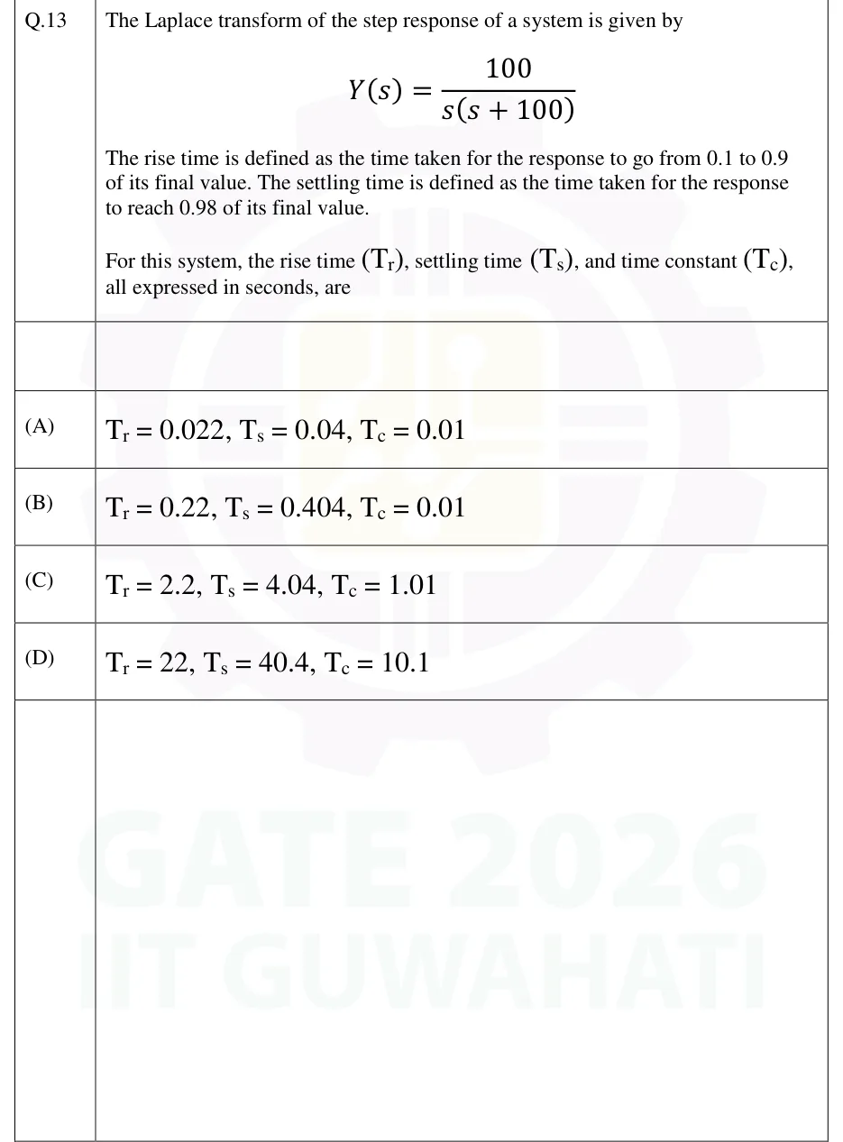
GATE 2026 EE Q.13

GATE 2026 · EEQ.13 · 1 mark · MCQ

The Laplace transform of the step response of a system is given by

The rise time is defined as the time taken for the response to go from 0.1 to 0.9 of its final value. The settling time is defined as the time taken for the response to reach 0.98 of its final value.

For this system, the rise time , settling time , and time constant , all expressed in seconds, are

  1. (A)

  2. (B)

  3. (C)

  4. (D)

Answer and solution
See the question in the paper
GATE 2026 EE Q.13: answer and solution

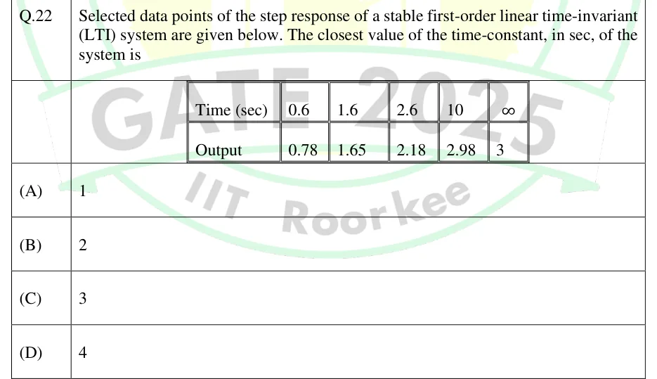
GATE 2025 EE Q.22

GATE 2025 · EEQ.22 · 1 mark · MCQ

Selected data points of the step response of a stable first-order linear time-invariant (LTI) system are given below. The closest value of the time-constant, in sec, of the system is

| Time (sec) | 0.6 | 1.6 | 2.6 | 10 | |
|---|---|---|---|---|---|
| Output | 0.78 | 1.65 | 2.18 | 2.98 | 3 |

  1. (A)

    1

  2. (B)

    2

  3. (C)

    3

  4. (D)

    4

Answer and solution
See the question in the paper
GATE 2025 EE Q.22: answer and solution

GATE 2025 IN Q.59

GATE 2025 · INQ.59 · 2 marks · NAT

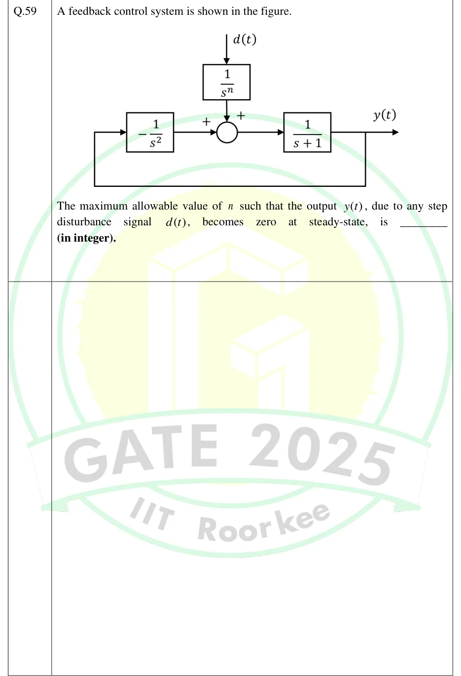
A feedback control system is shown in the figure.

The maximum allowable value of such that the output , due to any step disturbance signal , becomes zero at steady-state, is ________ (in integer).

GATE 2025 IN question 59: Block diagram with one summing junction, both inputs marked +.Tap to open full size
Figure from the GATE 2025 IN paper. It is part of the question.
Figure description

Block diagram with one summing junction, both inputs marked +. The disturbance d(t) enters from the top through a block 1/s^n and goes into the junction's top input (+). The junction output passes through a forward block 1/(s+1) to give the output y(t). y(t) is picked off and fed back along a path below the diagram to the left side, where it enters a feedback block -1/s^2 (the minus sign is inside the block). That block's output goes into the junction's left input (+). There is no separate reference input.

Answer and solution
GATE 2025 IN Q.59: answer and solution

GATE 2024 EC Q.13

GATE 2024 · ECQ.13 · 1 mark · MCQ

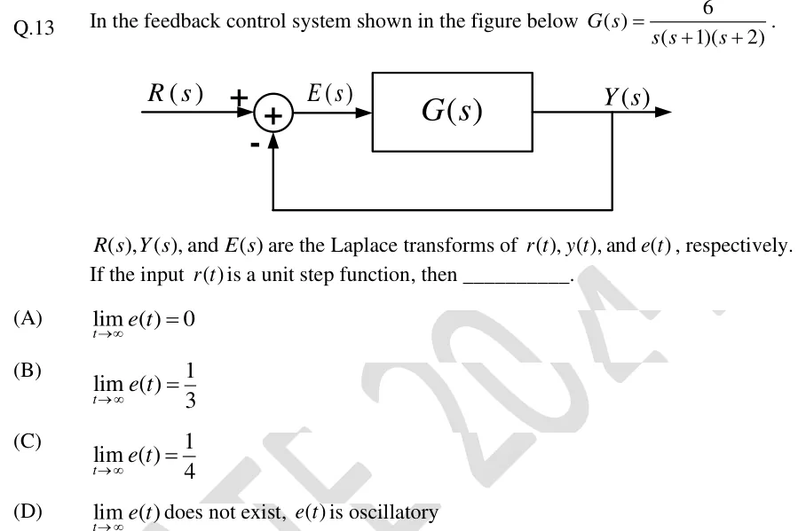
In the feedback control system shown in the figure below .

, , and are the Laplace transforms of , , and , respectively. If the input is a unit step function, then __________.

GATE 2024 EC question 13: Unity negative feedback loop.Tap to open full size
Figure from the GATE 2024 EC paper. It is part of the question.
Figure description

Unity negative feedback loop. Input R(s) enters a summing junction on its '+' terminal. The junction output E(s) feeds a block G(s), whose output is Y(s). Y(s) is taken off and fed back directly (gain 1, no block) to the summing junction's '-' terminal.

  1. (A)

  2. (B)

  3. (C)

  4. (D)

    does not exist, is oscillatory

Answer and solution
GATE 2024 EC Q.13: answer and solution

GATE 2024 EE Q.21

GATE 2024 · EEQ.21 · 1 mark · MCQ

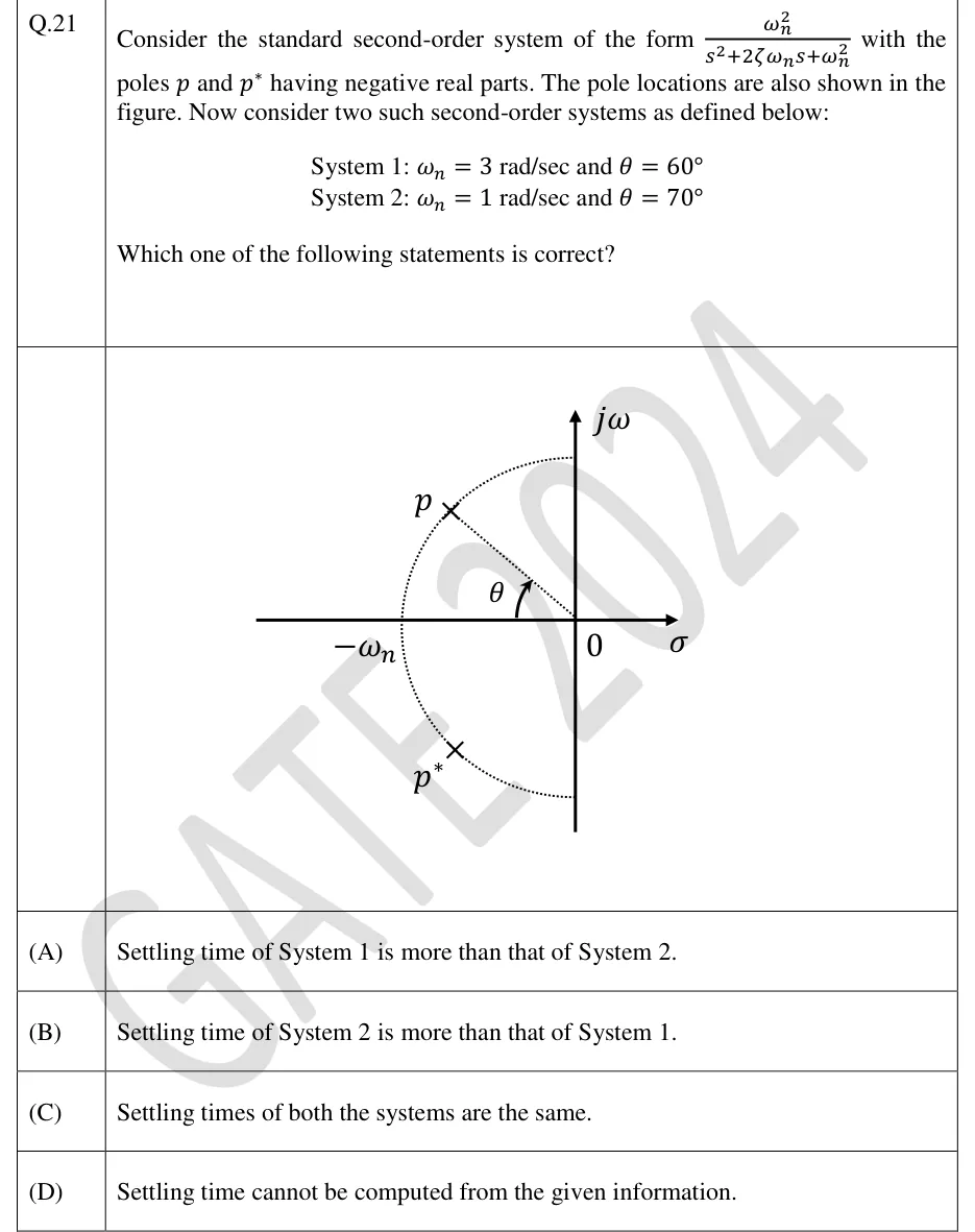
Consider the standard second-order system of the form with the poles and having negative real parts. The pole locations are also shown in the figure. Now consider two such second-order systems as defined below:

System 1: and

System 2: and

Which one of the following statements is correct?

GATE 2024 EE question 21: s-plane with horizontal axis labelled σ and vertical axis labelled j ω, origin marked 0.Tap to open full size
Figure from the GATE 2024 EE paper. It is part of the question.
Figure description

s-plane with horizontal axis labelled σ and vertical axis labelled j ω, origin marked 0. A dotted semicircle of radius ω_n centred at the origin lies in the left half-plane, meeting the negative real axis at the point labelled - ω_n and meeting the j ω axis above and below the origin. Pole p (cross) lies on the semicircle in the second quadrant and pole p^* (cross) is its mirror image in the third quadrant. A dotted line joins the origin to p; the angle θ is marked at the origin, measured between the negative real axis and this line.

  1. (A)

    Settling time of System 1 is more than that of System 2.

  2. (B)

    Settling time of System 2 is more than that of System 1.

  3. (C)

    Settling times of both the systems are the same.

  4. (D)

    Settling time cannot be computed from the given information.

Answer and solution
GATE 2024 EE Q.21: answer and solution

GATE 2024 EE Q.22

GATE 2024 · EEQ.22 · 1 mark · MCQ

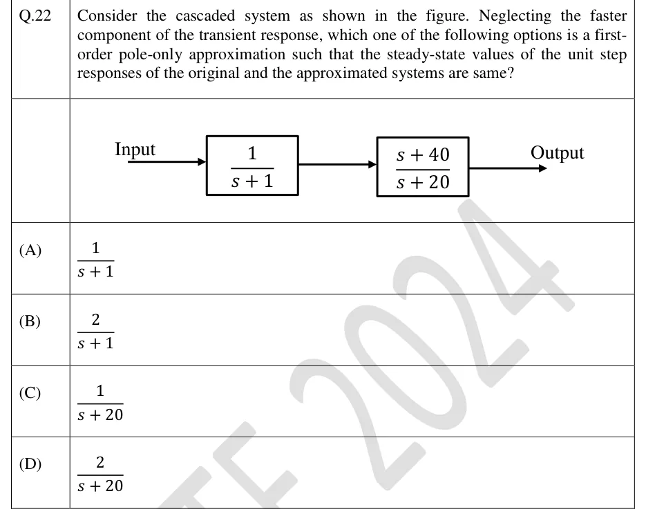
Consider the cascaded system as shown in the figure. Neglecting the faster component of the transient response, which one of the following options is a first-order pole-only approximation such that the steady-state values of the unit step responses of the original and the approximated systems are same?

GATE 2024 EE question 22: Two blocks in cascade (series), no feedback.Tap to open full size
Figure from the GATE 2024 EE paper. It is part of the question.
Figure description

Two blocks in cascade (series), no feedback. An arrow labelled "Input" enters the first block (1)/(s+1); its output arrow goes into the second block (s+40)/(s+20); the output arrow of the second block is labelled "Output".

  1. (A)

  2. (B)

  3. (C)

  4. (D)

Answer and solution
GATE 2024 EE Q.22: answer and solution

GATE 2024 IN Q.44

GATE 2024 · INQ.44 · 2 marks · MCQ

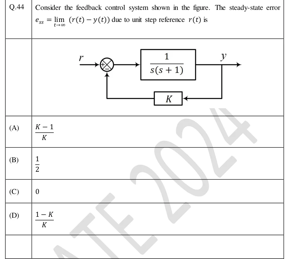
Consider the feedback control system shown in the figure. The steady-state error due to unit step reference is

GATE 2024 IN question 44: Block diagram: reference r enters a summing junction with sign + on the reference input and sign − on the feedback input.Tap to open full size
Figure from the GATE 2024 IN paper. It is part of the question.
Figure description

Block diagram: reference r enters a summing junction with sign + on the reference input and sign − on the feedback input. The junction output drives a forward block (1)/(s(s+1)) whose output is y. y is picked off and fed back through a block of gain K to the − input of the summing junction (non-unity negative feedback).

  1. (A)

  2. (B)

  3. (C)

  4. (D)

Answer and solution
GATE 2024 IN Q.44: answer and solution

GATE 2024 IN Q.45

GATE 2024 · INQ.45 · 2 marks · MCQ

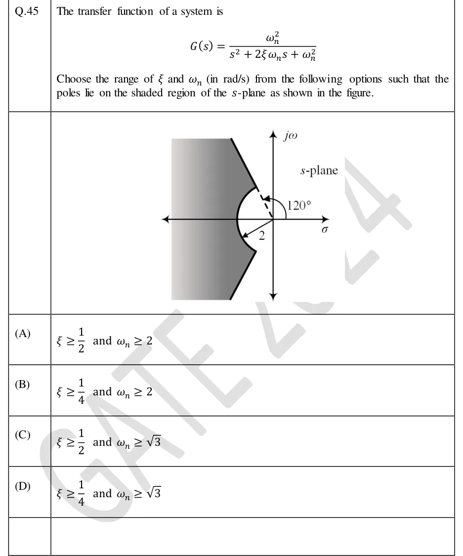
The transfer function of a system is

Choose the range of and (in rad/s) from the following options such that the poles lie on the shaded region of the -plane as shown in the figure.

GATE 2024 IN question 45: An s-plane with a vertical jω axis and a horizontal σ axis, both drawn with arrows, and the label 's-plane' in the first…Tap to open full size
Figure from the GATE 2024 IN paper. It is part of the question.
Figure description

An s-plane with a vertical jω axis and a horizontal σ axis, both drawn with arrows, and the label 's-plane' in the first quadrant. A dashed line runs from the origin into the second quadrant at 120° from the positive σ axis, and an arc marked 120° runs from the positive σ axis to it. The dashed line ends where it meets a solid circular arc of radius 2 centred at the origin. From there a solid ray continues outward along the same 120° direction. The arc runs through the left half-plane, crosses the negative real axis at −2, and ends at the mirror-image point in the third quadrant (at 240°, i.e. −120°; this angle is not labelled). From that point a second solid ray runs outward along the 240° direction. The lower ray is not drawn inside the arc. An arrow labelled 2 goes from the origin to the arc a little below the negative real axis, marking the radius. The shaded region lies outside the arc and between the two solid rays, so it contains the negative real axis beyond −2. It extends to the left edge of the figure, and the shading gets lighter towards the left. The region inside the arc near the origin is unshaded, and so is everything to the right of the rays.

  1. (A)

    and

  2. (B)

    and

  3. (C)

    and

  4. (D)

    and

Answer and solution
GATE 2024 IN Q.45: answer and solution

GATE 2023 EC Q.41

GATE 2023 · ECQ.41 · 2 marks · MCQ

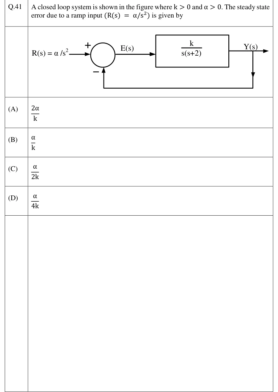
A closed loop system is shown in the figure where and . The steady state error due to a ramp input is given by

GATE 2023 EC question 41: Unity negative feedback loop.Tap to open full size
Figure from the GATE 2023 EC paper. It is part of the question.
Figure description

Unity negative feedback loop. Input R(s) = α /s^2 enters a summing junction with a + sign on the input and a − sign on the feedback path. The junction output is labelled E(s) and feeds a forward block (k)/(s(s+2)), whose output is Y(s). Y(s) is taken straight back, with no block in the path (unity gain), to the − input of the summing junction.

  1. (A)

  2. (B)

  3. (C)

  4. (D)

Answer and solution
GATE 2023 EC Q.41: answer and solution

GATE 2022 EC Q.50

GATE 2022 · ECQ.50 · 2 marks · MSQ

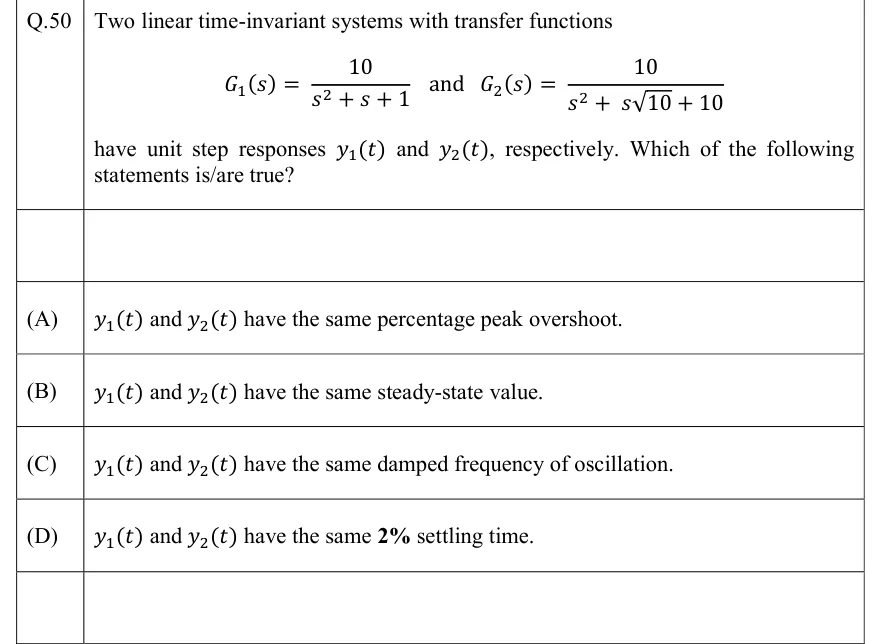
Two linear time-invariant systems with transfer functions

have unit step responses and , respectively. Which of the following statements is/are true?

  1. (A)

    and have the same percentage peak overshoot.

  2. (B)

    and have the same steady-state value.

  3. (C)

    and have the same damped frequency of oscillation.

  4. (D)

    and have the same settling time.

Answer and solution
See the question in the paper
GATE 2022 EC Q.50: answer and solution

GATE 2022 EC Q.60

GATE 2022 · ECQ.60 · 2 marks · NAT

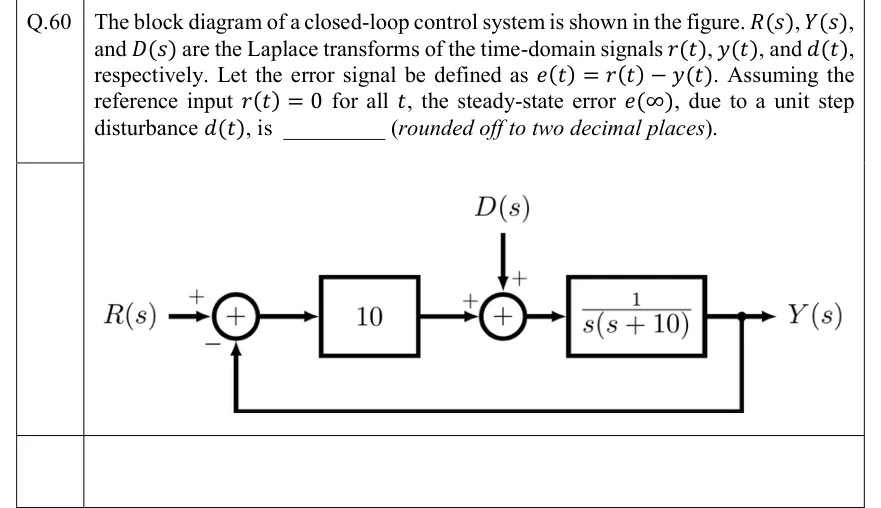
The block diagram of a closed-loop control system is shown in the figure. , , and are the Laplace transforms of the time-domain signals , , and , respectively. Let the error signal be defined as . Assuming the reference input for all , the steady-state error , due to a unit step disturbance , is ________ (rounded off to two decimal places).

GATE 2022 EC question 60: Unity-feedback loop.Tap to open full size
Figure from the GATE 2022 EC paper. It is part of the question.
Figure description

Unity-feedback loop. R(s) enters a summing junction with sign +; the feedback from Y(s) enters the same junction with sign −. The junction output (the error) passes through a gain block 10. The output of the gain block enters a second summing junction with sign +; the disturbance D(s) enters this second junction from above with sign +. The second junction output drives the plant block (1)/(s(s+10)), whose output is Y(s). Y(s) is fed back directly (unity gain) to the negative input of the first summing junction.

Answer and solution
GATE 2022 EC Q.60: answer and solution

GATE 2022 EE Q.39

GATE 2022 · EEQ.39 · 2 marks · MCQ

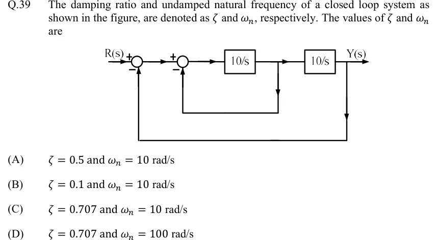
The damping ratio and undamped natural frequency of a closed loop system as shown in the figure, are denoted as and , respectively. The values of and are

GATE 2022 EE question 39: Block diagram: R(s) enters summing junction 1 (R with +, feedback with −).Tap to open full size
Figure from the GATE 2022 EE paper. It is part of the question.
Figure description

Block diagram: R(s) enters summing junction 1 (R with +, feedback with −). Output of junction 1 enters summing junction 2 (+ from junction 1, − from inner feedback). Output of junction 2 feeds block 10/s. Output of 10/s (a take-off point) feeds block 10/s, whose output is Y(s). Inner loop: unity negative feedback from the output of the first 10/s block back to the − input of junction 2. Outer loop: unity negative feedback from Y(s) back to the − input of junction 1.

  1. (A)

    and rad/s

  2. (B)

    and rad/s

  3. (C)

    and rad/s

  4. (D)

    and rad/s

Answer and solution
GATE 2022 EE Q.39: answer and solution

GATE 2022 IN Q.41

GATE 2022 · INQ.41 · 2 marks · MCQ

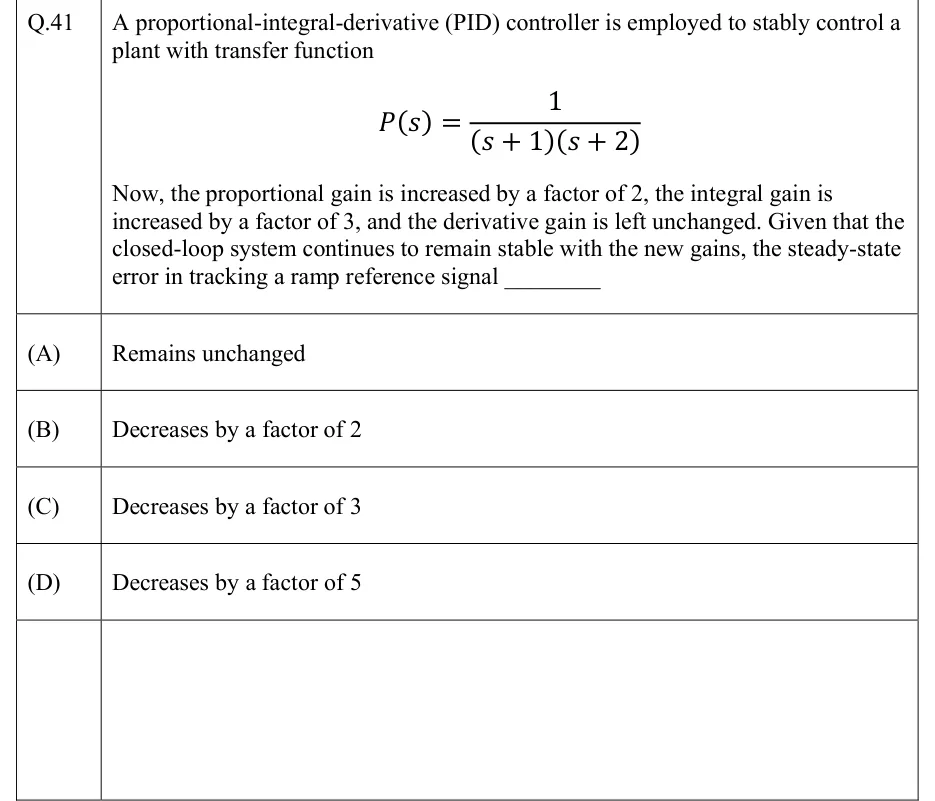
A proportional-integral-derivative (PID) controller is employed to stably control a plant with transfer function

Now, the proportional gain is increased by a factor of 2, the integral gain is increased by a factor of 3, and the derivative gain is left unchanged. Given that the closed-loop system continues to remain stable with the new gains, the steady-state error in tracking a ramp reference signal ________

  1. (A)

    Remains unchanged

  2. (B)

    Decreases by a factor of 2

  3. (C)

    Decreases by a factor of 3

  4. (D)

    Decreases by a factor of 5

Answer and solution
See the question in the paper
GATE 2022 IN Q.41: answer and solution

GATE 2020 EC Q.55

GATE 2020 · ECQ.55 · 2 marks · NAT

Consider the following closed loop control system

[Figure]

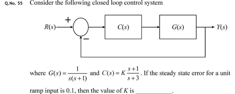
where and . If the steady state error for a unit ramp input is 0.1, then the value of is ________.

GATE 2020 EC question 55: Unity negative feedback loop.Tap to open full size
Figure from the GATE 2020 EC paper. It is part of the question.
Figure description

Unity negative feedback loop. Input R(s) enters a summing junction with a + sign on the reference input and a - sign on the feedback input. The summer output (error) feeds block C(s), which feeds block G(s) in cascade; the output of G(s) is Y(s). Y(s) is fed back directly (gain 1, no block) to the minus input of the summing junction.

Answer and solution
GATE 2020 EC Q.55: answer and solution

GATE 2020 EE Q.34

GATE 2020 · EEQ.34 · 2 marks · MCQ

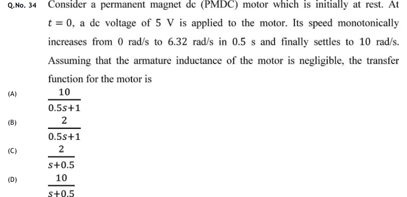
Consider a permanent magnet dc (PMDC) motor which is initially at rest. At , a dc voltage of is applied to the motor. Its speed monotonically increases from to in and finally settles to . Assuming that the armature inductance of the motor is negligible, the transfer function for the motor is

  1. (A)

  2. (B)

  3. (C)

  4. (D)

Answer and solution
See the question in the paper
GATE 2020 EE Q.34: answer and solution

GATE 2020 IN Q.37

GATE 2020 · INQ.37 · 2 marks · NAT

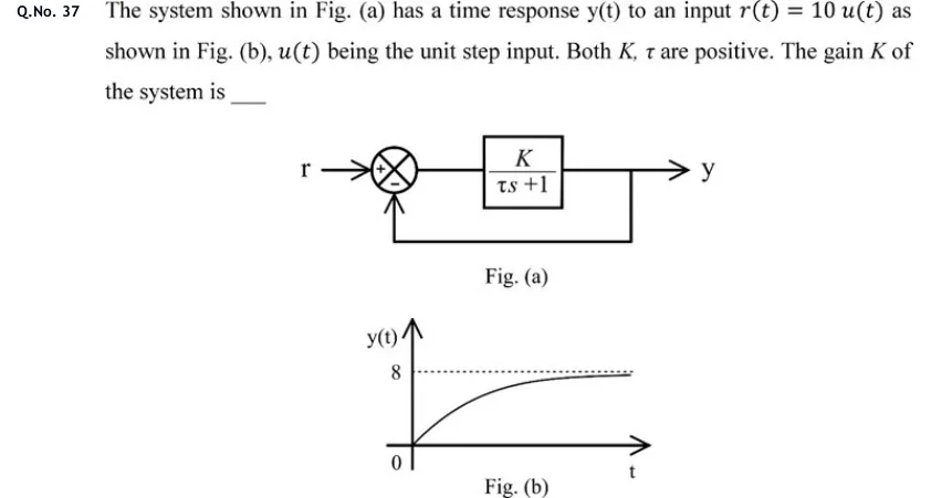
The system shown in Fig. (a) has a time response y(t) to an input as shown in Fig. (b), being the unit step input. Both , are positive. The gain of the system is ____

GATE 2020 IN question 37: Fig.Tap to open full size
Figure from the GATE 2020 IN paper. It is part of the question.
Figure description

Fig. (a): Block diagram. Input r enters a summing junction with sign +; the junction output feeds a forward block (K)/(τ s + 1) whose output is y. The output y is fed back directly (unity feedback, no block) to the summing junction with sign −. Fig. (b): Plot of y(t) versus t. Vertical axis labelled y(t) with marks 0 and 8; horizontal axis t. The curve starts at the origin (y = 0 at t = 0) and rises as a first-order exponential with no overshoot, approaching a dashed horizontal asymptote at y = 8.

Answer and solution
GATE 2020 IN Q.37: answer and solution

GATE 2018 EE Q.9

GATE 2018 · EEQ.9 · 1 mark · MCQ

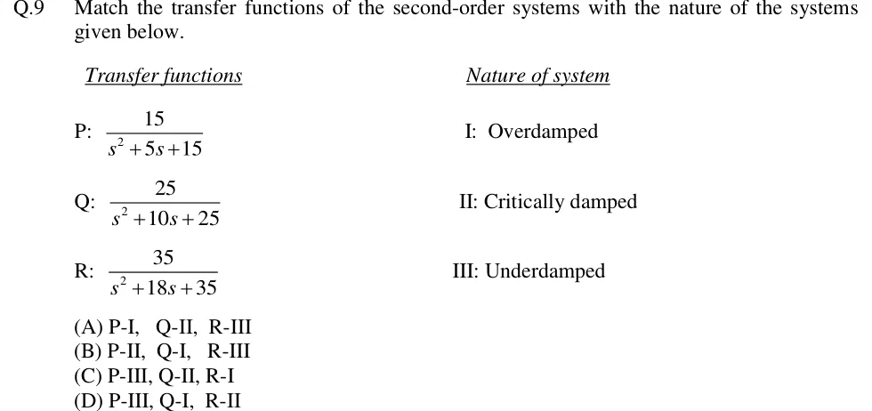
Match the transfer functions of the second-order systems with the nature of the systems given below.

Transfer functions

P:

Q:

R:

Nature of system

I: Overdamped

II: Critically damped

III: Underdamped

  1. (A)

    P-I, Q-II, R-III

  2. (B)

    P-II, Q-I, R-III

  3. (C)

    P-III, Q-II, R-I

  4. (D)

    P-III, Q-I, R-II

Answer and solution
See the question in the paper
GATE 2018 EE Q.9: answer and solution

GATE 2018 EE Q.46

GATE 2018 · EEQ.46 · 2 marks · NAT

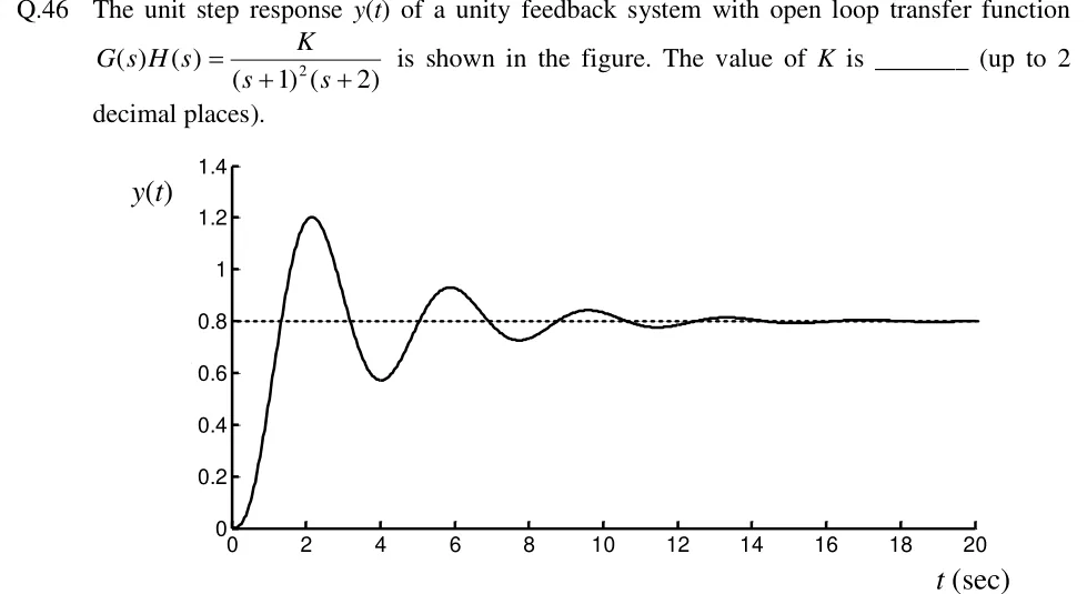
The unit step response of a unity feedback system with open loop transfer function is shown in the figure. The value of is _______ (up to 2 decimal places).

GATE 2018 EE question 46: Plot of y(t) (vertical axis, 0 to 1.4 in steps of 0.2) against t (sec) (horizontal axis, 0 to 20 in steps of 2).Tap to open full size
Figure from the GATE 2018 EE paper. It is part of the question.
Figure description

Plot of y(t) (vertical axis, 0 to 1.4 in steps of 0.2) against t (sec) (horizontal axis, 0 to 20 in steps of 2). The response starts at 0 and rises to a first peak of about 1.2 at t ≈ 2.2 s, falls to a minimum of about 0.57 at t ≈ 4 s, peaks again near 0.93 at t ≈ 5.9 s, dips to about 0.72 near t ≈ 7.7 s, peaks near 0.84 at t ≈ 9.6 s, and so on: a decaying oscillation that settles by t ≈ 16–20 s. A horizontal dashed line at y = 0.8 marks the steady-state value.

Answer and solution
GATE 2018 EE Q.46: answer and solution

PRACTICE

6 questions to test yourself

PRACTICE 11 mark · MCQ

A unity negative-feedback system has open-loop transfer function . For a unit-step input, what are the steady-state error and the 2% settling time of the closed-loop response (take )?

  1. (A)

    0.2 and 0.8 s

  2. (B)

    0.25 and 4 s

  3. (C)

    0.2 and 4 s

  4. (D)

    0 and 0.8 s

Answer and solution

Answer: (A)

  1. Closed loop: , which has one pole at . So s and s.

  2. The system is type 0 with , so .

  3. Check: , and . Using the open-loop pole instead ( s) would give the wrong settling time of 4 s.

PRACTICE 21 mark · NAT

A closed-loop system has . Using the dominant-pole approximation and , find the 2% settling time of the unit-step response, in seconds.

Answer and solution

Answer: (accepted range )

  1. The poles are at and . The real pole is 10 times further left than the complex pair, so it can be neglected.

  2. The reduced model, with DC gain kept at , is .

  3. From , , so s.

  4. This is the value the stated approximations give. Computing the exact responses gives about 2.11 s for the reduced model and about 2.16 s for the full third-order system.

PRACTICE 32 marks · NAT

A unity negative-feedback system has , with and . The unit-step response must have a peak overshoot of exactly (about 4.32%) and a 2% settling time of 1 s, where . Find .

Answer and solution

Answer: (accepted range )

  1. Closed loop: , so and .

  2. Setting gives , so .

  3. From , , so rad/s.

  4. . (Also, .)

PRACTICE 42 marks · MCQ

In a negative-feedback system, the forward path is and the feedback path is . The error is defined as . For a unit-step input , what is the steady-state value of ?

  1. (A)

    0.286

  2. (B)

    -0.429

  3. (C)

    0.429

  4. (D)

    0

Answer and solution

Answer: (B)

  1. Closed loop: . Its only pole is at , so it is stable.

  2. , which gives .

  3. Check with the equivalent unity loop: , so and .

  4. has a pole at , but that does not matter. The final value theorem needs the closed loop to be stable, and it is.

  5. Option A, , is the steady-state actuating error , not .

PRACTICE 52 marks · MSQ

A unity negative-feedback system has . Which of the following statements are correct?

  1. (A)

    The closed-loop system is stable.

  2. (B)

    The steady-state error to a unit-step input is zero.

  3. (C)

    The steady-state error to the input is 2.

  4. (D)

    The steady-state error to the input is 0.5.

Answer and solution

Answer: (A), (B), (C)

  1. Characteristic equation: . In the Routh array the entry is and the first column is all positive, so the loop is stable. A is correct.

  2. The system is type 1, so and the step error is 0. B is correct.

  3. , so the error for is . C is correct.

  4. For a type-1 system , so the parabolic error is infinite. D is wrong.

PRACTICE 62 marks · NAT

A unity negative-feedback loop has a proportional controller followed by a plant . A unit-step disturbance is added at the plant input (between the controller and the plant), and the reference is . With error defined as , find the steady-state value of .

Answer and solution

Answer: (accepted range )

  1. Transfer function from disturbance to output: . Its poles are at , so the loop is stable and the final value theorem applies.

  2. .

  3. With , . This matches .

  4. The plant's integrator does not remove this error, because it sits after the point where the disturbance enters. Answering 0 because the loop is type 1 is the trap.

OFFICIAL GATE 2027 SYLLABUS WORDING

Copied from the GATE 2027 syllabus; see all 2027 syllabi.

GATE EC

Transient and steady-state analysis of LTI systems

GATE EE

Transient and Steady‐state analysis of linear time invariant systems

GATE IN

transient response, steady state error

Preparing in Kolkata? IAE Academy's course for GATE ECE, GATE EE or GATE IN.