GATE EC · EE · IN

Root locus

The root locus shows where the closed-loop poles of a negative-feedback system move in the $s$ -plane as the loop gain $K$ goes from $0$ to $\infty$ . It comes from two facts: the angle condition, which decides whether a point lies on the locus, and the magnitude condition, which gives $K$ at that point. From these you can read off the range of $K$ for stability, the $j ω$ -crossing frequency, the gain for a required damping ratio, and how adding a pole or zero reshapes the response. With small changes, the same rules cover positive feedback (the complementary locus) and a parameter other than the gain.

7 previous-year questions · 7 solved · 6 practice questions

What the root locus is: the angle and magnitude conditions

For a negative-feedback loop whose open-loop transfer function is $K G (s) H (s)$ , the closed-loop poles are the roots of $1 + K G (s) H (s) = 0$ . The root locus is the path these roots trace in the $s$ -plane as the gain $K$ goes from $0$ to $\infty$ . The closed-loop poles decide stability, damping and speed of response. So one sketch tells you the stable range of $K$ , the gain that gives a required damping ratio, and what an added pole or zero does.

Convention used throughout these notes. $G (s) H (s)$ is written in pole-zero form with every factor monic, $G (s) H (s) = \frac{N ( s )}{D ( s )} = \frac{( s - z _{1} ) ( s - z _{2} ) \dots ( s - z _{m} )}{( s - p _{1} ) ( s - p _{2} ) \dots ( s - p _{n} )}$ . That way all of the gain sits in $K$ , and $K \geq 0$ . There are $n$ finite open-loop poles and $m$ finite open-loop zeros, with $n \geq m$ . Angles are measured counter-clockwise from the positive real axis, on vectors drawn from each pole or zero to the test point $s$ .

The locus shows poles only. With $K$ in the forward path, the closed-loop transfer function is $\frac{K G ( s )}{1 + K G ( s ) H ( s )}$ . Its zeros are the zeros of $G (s)$ and the poles of $H (s)$ , unless they cancel; for unity feedback they are just the open-loop zeros. These closed-loop zeros do not move as $K$ changes, and the root locus does not show them.

CLOSED-LOOP CHARACTERISTIC EQUATION

1 + K G (s) H (s) = 0 ⟺ D (s) + K N (s) = 0

Negative feedback, with $G (s) H (s) = N (s) / D (s)$ in monic form. The ordinary root locus is for $K \geq 0$ .

ANGLE CONDITION

∠ G (s) H (s) = j = 1 \sum m ∠ (s - z_{j}) - i = 1 \sum n ∠ (s - p_{i}) = \pm (2 q + 1) 18 0^{\circ}, q = 0, 1, 2, \dots

A point $s$ that is not itself an open-loop pole or zero is on the root locus ( $K \geq 0$ ) if and only if the net angle is an odd multiple of $18 0^{\circ}$ . $K$ does not appear, so this condition alone decides the shape of the locus.

MAGNITUDE CONDITION (GAIN AT A POINT)

K = \frac{1}{∣ G ( s ) H ( s ) ∣} = \frac{\prod _{i = 1}^{n} ∣ s - p _{i} ∣}{\prod _{j = 1}^{m} ∣ s - z _{j} ∣}

Use this only at a point that already satisfies the angle condition. It is the product of the distances to all poles divided by the product of the distances to all zeros. If $m = 0$ the denominator is $1$ .

EXAM TIP

Put the gain in root-locus form first. A loop given in time-constant form, e.g. $\frac{K ^{'} ( 1 + s /2 )}{s ( 1 + s /5 )}$ , equals $\frac{2.5 K ^{'} ( s + 2 )}{s ( s + 5 )}$ . The magnitude condition returns the root-locus gain $K = 2.5 K^{'}$ , not $K^{'}$ . If you skip this conversion, every gain you report is off by a constant factor, even when the sketch itself is correct.

Construction rules, in order

Apply the rules in this order, because each one uses the results of the ones before it. Rules 1 to 4 give the rough shape. Rules 5 to 9 fix the key numbers: the centroid, the breakaway points, the $j ω$ crossing, the departure angles and the gains.

1. Symmetry. The locus is symmetric about the real axis, because complex closed-loop poles come in conjugate pairs.
2. Number of branches. There are $max (n, m)$ branches, which is $n$ for a proper loop transfer function.
3. Start and end points. Each branch starts ( $K = 0$ ) at an open-loop pole and ends ( $K \to \infty$ ) at an open-loop zero. $m$ branches end at the finite zeros, and the other $n - m$ go to infinity along asymptotes.
4. Real-axis segments. A point on the real axis is on the locus if the total number of real open-loop poles and real zeros to its right is odd. Ignore complex-conjugate poles and zeros in this count, because their angles cancel. A repeated pole or zero counts as many times as its multiplicity.
5. Asymptotes. There are $n - m$ asymptotes, at angles $(2 q + 1) 18 0^{\circ} / (n - m)$ , all starting from the centroid $σ_{A}$ on the real axis.
6. Breakaway and break-in points. Solve $d K / d s = 0$ , with $K = - D (s) / N (s)$ taken from the characteristic equation. Keep only the roots that actually lie on the locus, i.e. those that give a real, positive $K$ . A breakaway point usually lies between two adjacent poles on a locus segment. A break-in point usually lies between two adjacent zeros, or between a zero and $- \infty$ .
7. Imaginary-axis crossing. Build the Routh array of $D (s) + K N (s)$ . The positive $K$ that makes a whole row zero (normally the $s^{1}$ row) is the marginal gain $K_{ma r}$ . The auxiliary equation from the row above, evaluated at $K_{ma r}$ , gives the crossing frequency. Check that its roots are purely imaginary, because a zero row can also mean a pair of real roots at $\pm σ$ . A zero $s^{0}$ row at $K = 0$ only marks an open-loop pole at the origin; it is not a crossing. Another way: substitute $s = j ω$ and set the real and imaginary parts to zero separately.
8. Angles of departure and arrival. At each complex pole, find the direction in which the branch leaves. At each complex zero, find the direction in which it arrives. Both come from applying the angle condition at a point very close to that pole or zero. Use the simple-pole formulas below, or the multiplicity form for a repeated pole.
9. Gain at any point. The magnitude condition gives $K$ at any point on the locus: a breakaway point, the $j ω$ crossing (a useful check against Routh), or where a constant- $ζ$ line cuts the locus.

NUMBER OF BRANCHES

N_{branches} = max (n, m)

$n$ is the number of finite open-loop poles and $m$ the number of finite zeros. For $n \geq m$ there are $n$ branches, and $n - m$ of them go to infinity.

ASYMPTOTE ANGLES

θ_{q} = \frac{( 2 q + 1 ) 18 0 ^{\circ}}{n - m}, q = 0, 1, \dots, (n - m - 1)

For $K \geq 0$ . Angles are measured counter-clockwise from the positive real axis. There are exactly $n - m$ asymptotes.

CENTROID (WHERE THE ASYMPTOTES MEET)

σ_{A} = \frac{\sum _{i = 1}^{n} p _{i} - \sum _{j = 1}^{m} z _{j}}{n - m}

Use the signed values: a pole at $- 3$ contributes $- 3$ . The imaginary parts of conjugate pairs cancel, so $σ_{A}$ is always real. You only need it when $n - m \geq 2$ . When $n - m = 1$ , the single asymptote is the negative real axis.

BREAKAWAY / BREAK-IN CONDITION

\frac{d K}{d s} = 0 with K = - \frac{D ( s )}{N ( s )} ⟺ N (s) D^{'} (s) - D (s) N^{'} (s) = 0

The roots are only candidates. Keep a root only if it lies on the locus: a real root must sit on a valid real-axis segment, and $K$ must come out real and positive.

BREAKAWAY CONDITION, RECIPROCAL FORM

i = 1 \sum n \frac{1}{σ - p _{i}} = j = 1 \sum m \frac{1}{σ - z _{j}}

The same condition, written for a real point $σ$ that is not itself a pole or zero. Unlike the real-axis rule, complex poles and zeros must be included here: a conjugate pair $a \pm j b$ contributes $\frac{2 ( σ - a )}{( σ - a ) ^{2} + b ^{2}}$ . The right-hand side is $0$ when there are no finite zeros.

BRANCH DIRECTIONS AT A BREAKAWAY POINT

spacing between arriving and leaving branches = \frac{18 0 ^{\circ}}{r}

When $r$ branches meet at a point, the $2 r$ arriving and leaving directions are equally spaced. In the usual case of $r = 2$ on the real axis, the branches leave at $\pm 9 0^{\circ}$ , i.e. perpendicular to the axis.

ANGLE OF DEPARTURE FROM A SIMPLE COMPLEX POLE

ϕ_{d} = 18 0^{\circ} - i \neq = k \sum ∠ (p_{k} - p_{i}) + j = 1 \sum m ∠ (p_{k} - z_{j})

For a pole $p_{k}$ that is not repeated. Use the angles of the vectors drawn from every other pole and from every zero to $p_{k}$ . Add or subtract $36 0^{\circ}$ to bring the result into $(- 18 0^{\circ}, 18 0^{\circ}]$ . The conjugate pole departs at $- ϕ_{d}$ .

DEPARTURE FROM A REPEATED POLE (MULTIPLICITY R)

ϕ_{d} = \frac{18 0 ^{\circ} + l 36 0 ^{\circ} - \sum _{i} ∠ ( p _{k} - p _{i} ) + \sum _{j} ∠ ( p _{k} - z _{j} )}{r}, l = 0, 1, \dots, r - 1

For an open-loop pole $p_{k}$ , real or complex, repeated $r$ times: the $r$ branches leave in these $r$ directions. The first sum runs over the poles other than the $r$ coincident ones, and the second over all zeros. With $r = 1$ this is the simple-pole formula. Example: for $\frac{K}{s ^{2} ( s + 4 )}$ the double pole at the origin gives $ϕ_{d} = 9 0^{\circ}$ and $27 0^{\circ}$ (i.e. $\pm 9 0^{\circ}$ ), so both branches leave vertically.

ANGLE OF ARRIVAL AT A SIMPLE COMPLEX ZERO

ϕ_{a} = 18 0^{\circ} - j \neq = k \sum ∠ (z_{k} - z_{j}) + i = 1 \sum n ∠ (z_{k} - p_{i})

For a zero $z_{k}$ that is not repeated. Use the angles of the vectors drawn from every other zero and from every pole to $z_{k}$ . The conjugate zero has arrival angle $- ϕ_{a}$ .

IMAGINARY-AXIS CROSSING FROM THE ROUTH ARRAY

row of zeros at K = K_{ma r}; A (s) = a s^{2} + b = 0 \Rightarrow ω = \frac{b}{a}

$A (s)$ is the auxiliary polynomial from the row just above the zero row (usually the $s^{2}$ row), evaluated at $K_{ma r} > 0$ . $b$ usually depends on $K$ , so substitute $K_{ma r}$ before taking the square root. This is a crossing only if $b / a > 0$ at $K_{ma r}$ . If $b / a < 0$ , the zero row signals a pair of real roots $\pm - b / a$ instead.

$n - m$	Asymptote angles ( $K \geq 0$ )	Behaviour as $K \to \infty$
1	$18 0^{\circ}$	One branch runs to $- \infty$ along the negative real axis
2	$\pm 9 0^{\circ}$	Two branches approach the vertical line $Re (s) = σ_{A}$ . For large $K$ they are in the left half-plane if $σ_{A} < 0$ and in the right half-plane if $σ_{A} > 0$
3	$\pm 6 0^{\circ}, 18 0^{\circ}$	Two branches enter the right half-plane, so the loop is unstable for large $K$
4	$\pm 4 5^{\circ}, \pm 13 5^{\circ}$	Two branches enter the right half-plane, so the loop is unstable for large $K$

EXAM TIP

Two common slips on the real axis. (i) Complex poles and zeros never count when you test a real-axis segment. (ii) A repeated pole counts twice. For $\frac{K}{s ^{2} ( s + 4 )}$ , the segment $(- 4, 0)$ is not on the locus, because the double pole at the origin gives two poles to its right, an even number. Only $(- \infty, - 4)$ is.

EXAM TIP

Check every breakaway root before you accept it. $d K / d s = 0$ also returns points of the complementary locus (where $K$ would be negative), and sometimes complex roots. Substitute each candidate into $K = - D (s) / N (s)$ . A genuine breakaway point on the ordinary locus gives a real, positive $K$ .

EXAM TIP

The breakaway point is where $K$ peaks on its segment. On a real-axis segment between two adjacent poles, $K = 0$ at both ends and $K > 0$ in between, so the branches break away where $K$ is largest on that segment. On a segment between two zeros, or between a zero and $- \infty$ , $K \to \infty$ at both ends, and the break-in point is where $K$ is smallest. In worked example 1, $K$ on $(- 3, 0)$ peaks at $63 \approx 10.39$ at $s \approx - 1.27$ (compare $K = 10$ at $s = - 1$ ).

Worked example 1: a three-pole locus from start to finish

WORKED EXAMPLE

A unity negative-feedback system has $G (s) = \frac{K}{s ( s + 3 ) ( s + 6 )}$ , $K \geq 0$ . Find the real-axis segments, the asymptotes, the breakaway point and the gain there, the $j ω$ -axis crossing, and the range of $K$ for stability.

Solution

Poles are at $0, - 3, - 6$ ( $n = 3$ ), with no finite zeros ( $m = 0$ ). There are three branches, and all three go to infinity.
Real-axis segments. Any point in $(- 3, 0)$ has 1 pole to its right (odd), so it is on the locus. Any point in $(- 6, - 3)$ has 2 (even), so it is not. Any point in $(- \infty, - 6)$ has 3, so it is on the locus.
Asymptotes: $n - m = 3$ , at angles $6 0^{\circ}, 18 0^{\circ}, 30 0^{\circ}$ (i.e. $\pm 6 0^{\circ}$ and $18 0^{\circ}$ ). Centroid: $σ_{A} = \frac{0 - 3 - 6}{3} = - 3$ .
Breakaway: $K = - s (s + 3) (s + 6) = - (s^{3} + 9 s^{2} + 18 s)$ . Setting $\frac{d K}{d s} = - (3 s^{2} + 18 s + 18) = 0$ gives $s^{2} + 6 s + 6 = 0$ , so $s = - 3 \pm 3$ , i.e. $- 1.268$ or $- 4.732$ .
$- 4.732$ lies in $(- 6, - 3)$ , which is not on the locus, so reject it. The breakaway point is $s = - 3 + 3 \approx - 1.268$ , between the poles at $0$ and $- 3$ as expected.
Gain at breakaway, from the magnitude condition (product of the distances to the three poles): $K = ∣ s ∣ ∣ s + 3∣ ∣ s + 6∣ = (3 - 3) (3) (3 + 3) = 3 (9 - 3) = 63 \approx 10.39$ .
$j ω$ crossing. The characteristic equation is $s^{3} + 9 s^{2} + 18 s + K = 0$ . Routh array: $s^{3}$ : $1, 18$ ; $s^{2}$ : $9, K$ ; $s^{1}$ : $\frac{162 - K}{9}$ ; $s^{0}$ : $K$ . The $s^{1}$ row vanishes at $K_{ma r} = 162$ .
Auxiliary equation from the $s^{2}$ row: $9 s^{2} + 162 = 0$ , so $s = \pm j 18 = \pm j 32 \approx \pm j 4.24$ rad/s.
Check with the sum rule ( $n - m = 3 \geq 2$ ). The closed-loop poles always add up to $0 - 3 - 6 = - 9$ . The crossing pair adds up to $0$ , so at $K = 162$ the third pole is at $- 9$ . Indeed $s^{3} + 9 s^{2} + 18 s + 162 = (s + 9) (s^{2} + 18)$ .
The picture: branches start at $0$ and $- 3$ and meet at $- 1.268$ when $K \approx 10.4$ . They leave the real axis at $\pm 9 0^{\circ}$ , bend towards the $\pm 6 0^{\circ}$ asymptotes, and cross the $j ω$ -axis at $\pm j 4.24$ when $K = 162$ . The third branch runs from $- 6$ to $- \infty$ along the real axis.

Answer: Real-axis segments: $(- 3, 0)$ and $(- \infty, - 6)$ . Asymptotes at $\pm 6 0^{\circ}$ and $18 0^{\circ}$ from $σ_{A} = - 3$ . Breakaway at $s = - 3 + 3 \approx - 1.27$ , with $K = 63 \approx 10.4$ . $j ω$ crossing at $\pm j 32 \approx \pm j 4.24$ rad/s, with $K = 162$ . Stable for $0 < K < 162$ .

Worked example 2: complex poles, departure angle and gain at a point

WORKED EXAMPLE

A negative-feedback system has $G (s) H (s) = \frac{K ( s + 4 )}{s ^{2} + 4 s + 8}$ , $K \geq 0$ . (a) Find the angle of departure from the upper complex pole. (b) Find the break-in point and the gain there. (c) Show that $s = - 4 + j 22$ lies on the root locus, and find $K$ at that point.

Solution

The poles are the roots of $s^{2} + 4 s + 8 = 0$ : $p_{1, 2} = - 2 \pm j 2$ . The zero is at $z = - 4$ . With $n = 2$ and $m = 1$ , one branch ends at $- 4$ and the other goes to $- \infty$ along the single asymptote at $18 0^{\circ}$ .
Real-axis segment: only $(- \infty, - 4)$ , which has one real zero to its right. The complex poles do not count.
(a) Departure from $p_{1} = - 2 + j 2$ . The vector from the zero is $p_{1} - (- 4) = 2 + j 2$ , at angle $4 5^{\circ}$ . The vector from the other pole is $p_{1} - p_{2} = j 4$ , at angle $9 0^{\circ}$ . So $ϕ_{d} = 18 0^{\circ} - 9 0^{\circ} + 4 5^{\circ} = 13 5^{\circ}$ . The lower branch leaves $p_{2}$ at $- 13 5^{\circ}$ .
(b) $K = - \frac{s ^{2} + 4 s + 8}{s + 4}$ . Then $N D^{'} - D N^{'} = (s + 4) (2 s + 4) - (s^{2} + 4 s + 8) = s^{2} + 8 s + 8 = 0$ , so $s = - 4 \pm 22$ , i.e. $- 1.172$ or $- 6.828$ .
$- 1.172$ is not on a real-axis segment of the ordinary locus (it would need $K < 0$ ), so reject it. The break-in point is $s = - 4 - 22 \approx - 6.83$ .
Gain there: $K = \frac{∣ s - p _{1} ∣ ∣ s - p _{2} ∣}{∣ s + 4∣}$ . At $s = - 4 - 22$ : $∣ s + 4∣ = 22$ and $∣ s - p_{1} ∣ ∣ s - p_{2} ∣ = (s + 2)^{2} + 4 = (2 + 22)^{2} + 4 = 16 + 82$ . So $K = \frac{16 + 8 2}{2 2} = 4 + 42 \approx 9.66$ .
(c) Angle test at $s = - 4 + j 22$ . From the zero, the vector is $j 22$ , at angle $9 0^{\circ}$ . From $p_{1}$ , it is $- 2 + j (22 - 2) = - 2 + j 0.828$ , at angle $18 0^{\circ} - 22. 5^{\circ} = 157. 5^{\circ}$ . From $p_{2}$ , it is $- 2 + j (22 + 2) = - 2 + j 4.828$ , at angle $18 0^{\circ} - 67. 5^{\circ} = 112. 5^{\circ}$ .
Net angle $= 9 0^{\circ} - 157. 5^{\circ} - 112. 5^{\circ} = - 18 0^{\circ}$ . This is an odd multiple of $18 0^{\circ}$ , so the point is on the locus.
Magnitude condition: $∣ s - p_{1} ∣ = 4 + 0.686 = 2.165$ , $∣ s - p_{2} ∣ = 4 + 23.31 = 5.226$ and $∣ s + 4∣ = 2.828$ . So $K = \frac{2.165 \times 5.226}{2.828} = 4.0$ .
Check: $D (s) + K N (s) = s^{2} + (4 + K) s + (8 + 4 K)$ . With $K = 4$ this is $s^{2} + 8 s + 24$ , whose roots are $- 4 \pm j 22$ , as required.

Answer: (a) $ϕ_{d} = 13 5^{\circ}$ at $- 2 + j 2$ (and $- 13 5^{\circ}$ at $- 2 - j 2$ ). (b) Break-in at $s = - 4 - 22 \approx - 6.83$ , with $K = 4 + 42 \approx 9.66$ . (c) The point is on the locus, with $K = 4$ .

EXAM TIP

Two poles and one real zero give a circle. Take $G (s) H (s) = \frac{K ( s + c )}{D ( s )}$ with $D (s)$ quadratic and $c$ real. If $D (- c) > 0$ , any part of the locus off the real axis is an arc of the circle centred at the zero $s = - c$ with radius $r = D (- c)$ . $D (- c)$ is the product of the distances from the zero to the two poles. If the zero lies between two real poles, $D (- c) < 0$ and the whole locus stays on the real axis. The points $- c \pm r$ are exactly the roots of the breakaway equation, so keep only those on valid real-axis segments. With a complex pole pair, only $- c - r$ is valid (the break-in point). With the zero to the left of two real poles, both are valid: one breakaway point and one break-in point. With the zero to the right of both real poles, neither is valid, and the ordinary locus has no off-axis part. In example 2, $D (- 4) = 16 - 16 + 8 = 8$ , so $r = 22$ . The break-in point is $- 6.83$ , and $- 1.17$ belongs to the complementary locus.

Results that save time

SUM OF CLOSED-LOOP POLES (POLE EXCESS AT LEAST 2)

i = 1 \sum n r_{i} (K) = i = 1 \sum n p_{i} (n - m \geq 2)

When $n - m \geq 2$ , $K$ does not appear in the $s^{n - 1}$ coefficient of $D (s) + K N (s)$ , so the closed-loop poles $r_{i}$ always add up to the sum of the open-loop poles. Use it to find the remaining real pole at the $j ω$ crossing without dividing polynomials.

CONSTANT DAMPING-RATIO LINE

s = - ζ ω_{n} \pm j ω_{n} 1 - ζ^{2}, θ = cos^{- 1} ζ

For $0 < ζ < 1$ . Closed-loop poles with damping ratio $ζ$ lie on the two radial lines from the origin at angle $θ$ above and below the negative real axis. The gain for a required $ζ$ is $K$ , from the magnitude condition, at the point where this line cuts the locus. If the line cuts the locus more than once, each crossing gives a valid gain.

GAIN MARGIN READ FROM THE LOCUS

GM = \frac{K _{ma r}}{K _{design}}, G M_{d B} = 20 lo g_{10} \frac{K _{ma r}}{K _{design}}

Valid in the usual case where the loop is stable for $0 < K < K_{ma r}$ and becomes unstable once $K$ passes $K_{ma r}$ (a single $j ω$ crossing). Both gains must be in the same form. The ratio is the same whichever constant form is used.

EXAM TIP

Gain for a given damping ratio. Take $G (s) = \frac{K}{s ( s + 4 )}$ and $ζ = 0.5$ , so $θ = 6 0^{\circ}$ . The complex part of the locus is the vertical line $Re (s) = - 2$ , which meets the $6 0^{\circ}$ line at $s = - 2 + j 23$ . The distances to the poles at $0$ and $- 4$ are both $4$ , so $K = 4 \times 4 = 16$ . As a check, $s^{2} + 4 s + K$ with $2 ζ ω_{n} = 4$ gives $ω_{n} = 4$ and $K = ω_{n}^{2} = 16$ .

EXAM TIP

A pole excess of 3 or more always means instability at high gain. When $n - m \geq 3$ , the $q = 0$ asymptote makes an angle $18 0^{\circ} / (n - m) \leq 6 0^{\circ}$ with the positive real axis. So at least two asymptotes, this one and its mirror image, point into the right half-plane, and the loop cannot be stable for all $K > 0$ . It may be stable for $0 < K < K_{ma r}$ , or, as with $\frac{K}{s ^{2} ( s + 4 )}$ , for no $K$ at all.

EXAM TIP

Don't assume the stable range is 0 < K < K_mar. If the loop has an open-loop pole in the right half-plane, a branch starts there and may cross into the left half-plane as $K$ grows. The stable range is then $K > K_{1}$ , or $K_{1} < K < K_{2}$ . A locus that crosses the $j ω$ -axis more than once (a conditionally stable system) can also have separate stable ranges. An open-loop zero in the right half-plane pulls a branch into the right half-plane at high gain. Read the direction of each crossing from the sketch, or confirm with Routh.

Effect of adding poles and zeros

An added open-loop pole or zero changes $n - m$ , the centroid and the angle budget at every point, so the whole locus moves. As a rule of thumb, an added left-half-plane pole pushes the locus to the right (towards instability), and an added left-half-plane zero pulls it to the left (towards stability). The Routh checks below confirm this for two specific loops.

Change to $G (s) H (s)$	What happens to the locus	Effect on the closed loop
Add a LHP pole	$n - m$ rises by 1, the asymptote angles shrink (e.g. $\pm 9 0^{\circ} \to \pm 6 0^{\circ}$ ) and the centroid moves. Branches bend to the right.	Usually less relative stability and a more oscillatory response. A finite $K_{ma r}$ can appear where there was none. Compared at the same DC loop gain (the pole added as $\frac{1}{1 + s / a}$ ), an existing $K_{ma r}$ usually falls. For example, $\frac{K}{s ( s + 1 ) ( s + 2 )}$ has $K_{ma r} = 6$ , and an extra $\frac{10}{s + 10}$ lowers it to about $4.69$ .
Add a LHP zero	$n - m$ falls by 1. Branches bend to the left and are drawn towards the zero.	Usually more relative stability and a better-damped response. Can stabilise a loop that was unstable for every $K$ (see below).
Add a pole at the origin (integrator)	Same as adding a pole, at the left-half-plane location that adds the most phase lag.	System type rises by 1 (better steady-state accuracy), but relative stability usually drops.
Add a lead pair $\frac{s + a}{s + b}$ , $0 < a < b$	Net positive angle added. The locus moves left.	Usually better transient response and relative stability.
Add a lag pair $\frac{s + a}{s + b}$ , $0 < b < a$ , both near the origin	Shape of the locus almost unchanged away from the origin.	Higher low-frequency gain (smaller steady-state error), with the dominant poles nearly unchanged.

Two checks with the Routh test. $\frac{K}{s ( s + 2 )}$ gives $s^{2} + 2 s + K$ , which is stable for every $K > 0$ . Adding a pole at $- 4$ gives $s^{3} + 6 s^{2} + 8 s + K$ , which is stable only for $0 < K < 48$ . In the other direction, $\frac{K}{s ^{2} ( s + 4 )}$ gives $s^{3} + 4 s^{2} + K$ . The $s$ term is missing, so it is unstable for every $K > 0$ . Adding a zero at $- 1$ gives $s^{3} + 4 s^{2} + K s + K$ , whose $s^{1}$ Routh entry is $3 K /4 > 0$ , so it is stable for every $K > 0$ . In general, $\frac{K ( s + b )}{s ^{2} ( s + a )}$ is stable for all $K > 0$ exactly when $0 < b < a$ , i.e. the zero is closer to the origin than the pole.

Root locus for a parameter other than the gain

The construction rules only need the characteristic equation in the form $1 + (parameter) \times F (s) = 0$ , with the parameter non-negative. When the quantity that varies is not the loop gain (a pole location, a velocity-feedback gain, a controller coefficient), collect the terms that contain it and divide through by the rest. The resulting plot is sometimes called a root contour.

EQUIVALENT LOOP FOR A VARYING PARAMETER

Q (s) + α P (s) = 0 ⟺ 1 + α \frac{P ( s )}{Q ( s )} = 0

Valid when the characteristic polynomial is linear in the parameter $α \geq 0$ . Apply every rule to $P (s) / Q (s)$ with $α$ in place of $K$ . The poles of this equivalent loop are the roots of $Q (s)$ , i.e. the closed-loop poles at $α = 0$ . They are generally not the open-loop poles of the physical system. If $P (s)$ or $Q (s)$ is not monic, move the leading coefficients into the gain first.

WORKED EXAMPLE

A unity negative-feedback system has $G (s) = \frac{10}{s ( s + a )}$ , where the pole location $a \geq 0$ is the parameter that varies. Describe how the closed-loop poles move as $a$ goes from $0$ to $\infty$ , and find the value of $a$ that gives critical damping.

Solution

Characteristic equation: $s (s + a) + 10 = 0$ , i.e. $(s^{2} + 10) + a s = 0$ . Divide by the terms without $a$ : $1 + a \frac{s}{s ^{2} + 10} = 0$ .
Equivalent loop $a P (s) / Q (s)$ with $P (s) = s$ and $Q (s) = s^{2} + 10$ . Its poles are $\pm j 10$ (the closed-loop poles at $a = 0$ ), and it has one zero at $s = 0$ . With $n = 2$ and $m = 1$ , one branch ends at the origin and the other goes to $- \infty$ .
Real-axis segments: $(- \infty, 0)$ has one zero to its right, so it is on the locus. $(0, \infty)$ is not. The complex poles do not count.
Departure from $j 10$ . The vector from the zero is $j 10$ ( $9 0^{\circ}$ ) and the vector from the other pole is $j 210$ ( $9 0^{\circ}$ ). So $ϕ_{d} = 18 0^{\circ} - 9 0^{\circ} + 9 0^{\circ} = 18 0^{\circ}$ , and the branch leaves horizontally, to the left.
Break-in: $P Q^{'} - Q P^{'} = s (2 s) - (s^{2} + 10) = s^{2} - 10 = 0$ , so $s = \pm 10$ . Only $- 10 \approx - 3.16$ lies on the locus.
Parameter value there: $a = - \frac{Q ( s )}{P ( s )} = - \frac{10 + 10}{- 10} = 210 \approx 6.32$ .
Check: $s^{2} + 210 s + 10 = (s + 10)^{2}$ , a double root, so $ζ = 1$ . Also, $ω_{n}^{2} = 10$ for every $a$ . So for $0 < a < 210$ the poles move on the circle $∣ s ∣ = 10$ centred at the origin, as the two-poles-one-zero circle rule predicts ( $r^{2} = Q (0) = 10$ ).

Answer: The poles start at $\pm j 10$ and move left along the circle $∣ s ∣ = 10$ . They meet at $s = - 10$ when $a = 210 \approx 6.32$ , which is critical damping. They then split along the real axis, one towards the origin and one towards $- \infty$ .

Complementary (negative-K) root locus

Suppose $K$ runs from $0$ to $- \infty$ with negative feedback, or equivalently the loop has positive feedback with $K \geq 0$ , so that the characteristic equation is $1 - K G (s) H (s) = 0$ . Then the angle condition changes from odd to even multiples of $18 0^{\circ}$ . The locus you get is the complementary (inverse) root locus, and the ordinary and complementary loci together make the complete root locus. Every rule that depends on the $18 0^{\circ}$ condition changes. The rest stay the same.

ANGLE AND MAGNITUDE CONDITIONS, COMPLEMENTARY LOCUS

∠ G (s) H (s) = \pm q 36 0^{\circ}, q = 0, 1, 2, \dots ∣ K ∣ = \frac{\prod _{i = 1}^{n} ∣ s - p _{i} ∣}{\prod _{j = 1}^{m} ∣ s - z _{j} ∣}

Applies to $K \leq 0$ with negative feedback, or to $K \geq 0$ with positive feedback.

ASYMPTOTE ANGLES, COMPLEMENTARY LOCUS

θ_{q} = \frac{q 36 0 ^{\circ}}{n - m}, q = 0, 1, \dots, (n - m - 1)

The centroid formula does not change. When $n > m$ there is always an asymptote at $0^{\circ}$ , i.e. along the positive real axis.

Rule	Ordinary locus ( $K \geq 0$ )	Complementary locus ( $K \leq 0$ )
Angle condition	Odd multiple of $18 0^{\circ}$	Even multiple of $18 0^{\circ}$ ( $0^{\circ}, \pm 36 0^{\circ}, \dots$ )
Real-axis segment	Odd number of real poles and zeros to the right	Even number (including zero) to the right
Asymptote angles	$\frac{( 2 q + 1 ) 18 0 ^{\circ}}{n - m}$	$\frac{q 36 0 ^{\circ}}{n - m}$
$n - m = 3$ example	$\pm 6 0^{\circ}, 18 0^{\circ}$	$0^{\circ}, \pm 12 0^{\circ}$
Centroid, symmetry, number of branches, start and end points	As derived	Unchanged
Breakaway candidates	Roots of $d K / d s = 0$ giving $K > 0$	Roots of $d K / d s = 0$ giving $K < 0$
Departure angle (simple pole)	$18 0^{\circ} - \sum ∠_{poles} + \sum ∠_{zeros}$	$0^{\circ} - \sum ∠_{poles} + \sum ∠_{zeros}$

EXAM TIP

Positive feedback uses the complementary rules. A positive-feedback loop with $K \geq 0$ has characteristic equation $1 - K G (s) H (s) = 0$ . Its locus always has a branch heading along the positive real axis ( $0^{\circ}$ asymptote), so when $n > m$ it is unstable for large enough $K$ .

EXAM TIP

Where the rejected root goes. In worked example 2, the rejected root $- 4 + 22 \approx - 1.17$ gives $K = - \frac{D ( s )}{N ( s )} = 4 - 42 \approx - 1.66 < 0$ . It is where the two complementary branches from the complex poles meet on the real axis. From there, one branch runs to $+ \infty$ and the other to the zero at $- 4$ .

PREVIOUS-YEAR QUESTIONS

7 questions from the EC, EE and IN papers

Try each question first, then open the answer. We placed each question under a topic ourselves; the exam paper does not label topics.

See these papers in full: GATE ECE 2025 · GATE ECE 2022 · GATE ECE 2020 · GATE EE 2025 · GATE EE 2024 · GATE IN 2024 · GATE IN 2020

GATE 2025 EC Q.26

GATE 2025 · ECQ.26 · 1 mark · MSQ

Consider the unity-negative-feedback system shown in Figure (i) below, where gain $K \geq 0$ . The root locus of this system is shown in Figure (ii) below.

For what value(s) of $K$ will the system in Figure (i) have a pole at $- 1 + j 1$ ?

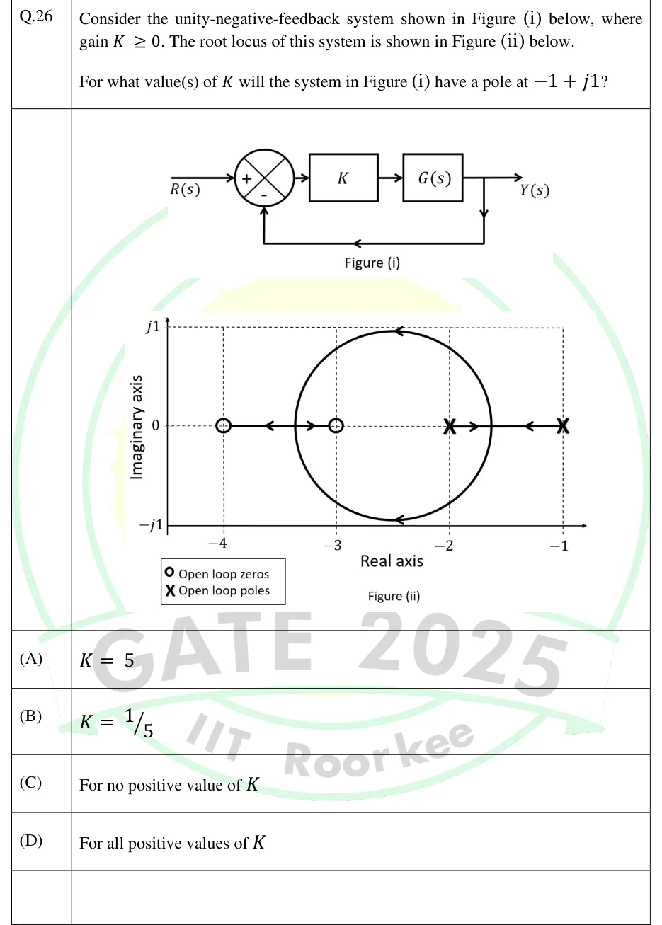
GATE 2025 EC question 26: Figure (i): block diagram. — Figure from the GATE 2025 EC paper. It is part of the question.

(A)
$K = 5$
(B)
$K = \frac{1}{5}$
(C)
For no positive value of $K$
(D)
For all positive values of $K$

Answer and solution

GATE 2025 EC Q.26: answer and solution

GATE 2025 EE Q.29

GATE 2025 · EEQ.29 · 1 mark · MSQ

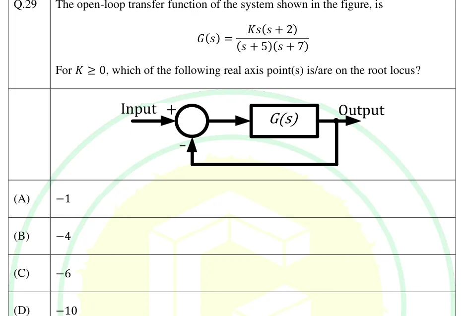
The open-loop transfer function of the system shown in the figure, is

G (s) = \frac{K s ( s + 2 )}{( s + 5 ) ( s + 7 )}

For $K \geq 0$ , which of the following real axis point(s) is/are on the root locus?

GATE 2025 EE question 29: Unity negative feedback loop. — Figure from the GATE 2025 EE paper. It is part of the question.

(A)
$- 1$
(B)
$- 4$
(C)
$- 6$
(D)
$- 10$

Answer and solution

GATE 2025 EE Q.29: answer and solution

GATE 2024 EE Q.57

GATE 2024 · EEQ.57 · 2 marks · NAT

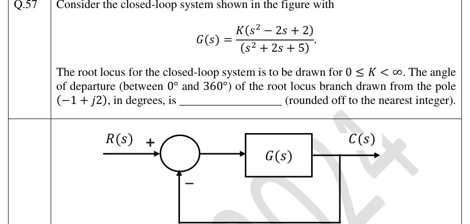
Consider the closed-loop system shown in the figure with
$G (s) = \frac{K ( s ^{2} - 2 s + 2 )}{( s ^{2} + 2 s + 5 )} .$
The root locus for the closed-loop system is to be drawn for $0 \leq K < \infty$ . The angle of departure (between $0^{\circ}$ and $36 0^{\circ}$ ) of the root locus branch drawn from the pole $(- 1 + j 2)$ , in degrees, is ________ (rounded off to the nearest integer).

GATE 2024 EE question 57: Unity negative feedback loop. — Figure from the GATE 2024 EE paper. It is part of the question.

Answer and solution

GATE 2024 EE Q.57: answer and solution

GATE 2024 IN Q.55

GATE 2024 · INQ.55 · 2 marks · NAT

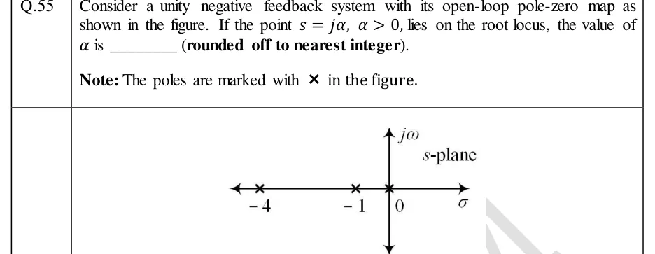
Consider a unity negative feedback system with its open-loop pole-zero map as shown in the figure. If the point $s = j α$ , $α > 0$ , lies on the root locus, the value of $α$ is ________ (rounded off to nearest integer).

Note: The poles are marked with $\times$ in the figure.

GATE 2024 IN question 55: s-plane pole-zero map: horizontal real axis labelled sigma (arrowheads both ends), vertical imaginary axis labelled… — Figure from the GATE 2024 IN paper. It is part of the question.

Answer and solution

GATE 2024 IN Q.55: answer and solution

GATE 2022 EC Q.22

GATE 2022 · ECQ.22 · 1 mark · MCQ

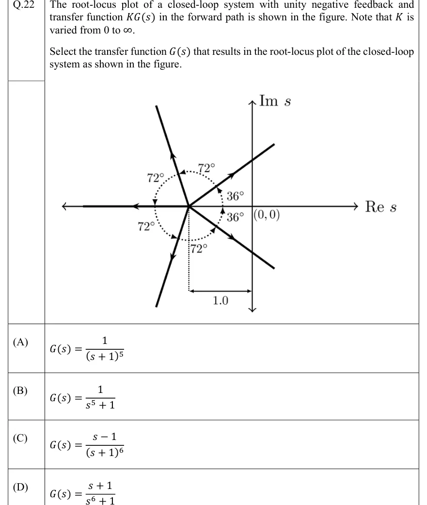
The root-locus plot of a closed-loop system with unity negative feedback and transfer function $K G (s)$ in the forward path is shown in the figure. Note that $K$ is varied from 0 to $\infty$ .

Select the transfer function $G (s)$ that results in the root-locus plot of the closed-loop system as shown in the figure.

GATE 2022 EC question 22: s-plane with horizontal axis 'Re s' and vertical axis 'Im s'. — Figure from the GATE 2022 EC paper. It is part of the question.

(A)
$G (s) = \frac{1}{( s + 1 ) ^{5}}$
(B)
$G (s) = \frac{1}{s ^{5} + 1}$
(C)
$G (s) = \frac{s - 1}{( s + 1 ) ^{6}}$
(D)
$G (s) = \frac{s + 1}{s ^{6} + 1}$

Answer and solution

GATE 2022 EC Q.22: answer and solution

GATE 2020 EC Q.40

GATE 2020 · ECQ.40 · 2 marks · MCQ

The characteristic equation of a system is

s^{3} + 3 s^{2} + (K + 2) s + 3 K = 0.

In the root locus plot for the given system, as $K$ varies from $0$ to $\infty$ , the break-away or break-in point(s) lie within

(A)
$(- 1, 0)$ .
(B)
$(- 2, - 1)$ .
(C)
$(- 3, - 2)$ .
(D)
$(- \infty, - 3)$ .

Answer and solution

GATE 2020 EC Q.40: answer and solution

See the question in the paper

Tap to open full size

GATE 2020 EC Q.40: answer and solution

GATE 2020 IN Q.36

GATE 2020 · INQ.36 · 2 marks · NAT

The loop transfer function of a negative feedback system is given by

G (s) H (s) = \frac{K}{s ( s + 2 ) ( s + 6 )},

where $K > 0$ . The value of $K$ at the breakaway point of the root locus for the above system (rounded off to one decimal place) is ____

Answer and solution

GATE 2020 IN Q.36: answer and solution

See the question in the paper

Tap to open full size

GATE 2020 IN Q.36: answer and solution

PRACTICE

6 questions to test yourself

PRACTICE 11 mark · MCQ

A negative-feedback system has $G (s) H (s) = \frac{K ( s + 5 )}{s ( s + 2 ) ( s + 8 ) ( s + 10 )}$ , $K \geq 0$ . The root-locus asymptotes meet the real axis at $σ_{A}$ and make angles $θ$ with the positive real axis. Which of the following is correct?

(A)
$σ_{A} = - 5$ ; $θ = \pm 6 0^{\circ}, 18 0^{\circ}$
(B)
$σ_{A} = - 6.67$ ; $θ = \pm 6 0^{\circ}, 18 0^{\circ}$
(C)
$σ_{A} = - 5$ ; $θ = \pm 4 5^{\circ}, \pm 13 5^{\circ}$
(D)
$σ_{A} = - 8.33$ ; $θ = \pm 6 0^{\circ}, 18 0^{\circ}$

Answer and solution

Answer: (A)

$n = 4$ poles ( $0, - 2, - 8, - 10$ ) and $m = 1$ zero ( $- 5$ ), so $n - m = 3$ asymptotes.
Angles: $(2 q + 1) 18 0^{\circ} /3 = 6 0^{\circ}, 18 0^{\circ}, 30 0^{\circ}$ , i.e. $\pm 6 0^{\circ}$ and $18 0^{\circ}$ .
$σ_{A} = \frac{( 0 - 2 - 8 - 10 ) - ( - 5 )}{3} = \frac{- 20 + 5}{3} = - 5$ .
B leaves out the zero ( $- 20/3$ ). D gets the sign of the zero wrong ( $(- 20 - 5) /3$ ). C uses $n$ instead of $n - m$ for the number of asymptotes.

PRACTICE 22 marks · NAT

A unity negative-feedback system has $G (s) = \frac{K}{s ( s + 2 ) ( s + 5 )}$ , $K \geq 0$ . At the value of $K$ where the root locus crosses the imaginary axis, the third (real) closed-loop pole is at $s = σ$ . The value of $σ$ is ______.

Answer and solution

Answer: $- 7$ (accepted range $\pm 0.01$ )

Characteristic equation: $s^{3} + 7 s^{2} + 10 s + K = 0$ .
Routh array: $s^{3}$ : $1, 10$ ; $s^{2}$ : $7, K$ ; $s^{1}$ : $\frac{70 - K}{7}$ ; $s^{0}$ : $K$ . So $K_{ma r} = 70$ .
Auxiliary equation: $7 s^{2} + 70 = 0$ , so $s = \pm j 10$ . These two poles add up to $0$ .
$n - m = 3 \geq 2$ , so the closed-loop poles always add up to $0 - 2 - 5 = - 7$ . Therefore $σ = - 7$ .
Check: $(s + 7) (s^{2} + 10) = s^{3} + 7 s^{2} + 10 s + 70$ .

PRACTICE 32 marks · MSQ

A negative-feedback system has $G (s) H (s) = \frac{K ( s + 1 )}{s ( s - 2 )}$ , $K \geq 0$ . Which of the following statements is/are TRUE?

(A)
The closed-loop system is stable for every $K > 2$ .
(B)
The root locus leaves the real axis at a breakaway point $s = - 1 + 3 \approx 0.732$ .
(C)
The root locus crosses the imaginary axis at $s = \pm j 2$ .
(D)
The real-axis segment between $s = - 1$ and $s = 0$ is part of the root locus.

Answer and solution

Answer: (A), (B)

Characteristic equation: $s (s - 2) + K (s + 1) = s^{2} + (K - 2) s + K = 0$ . A second-order polynomial is stable if and only if all its coefficients are positive, which here means $K > 2$ . A is true.
Breakaway: $N D^{'} - D N^{'} = (s + 1) (2 s - 2) - (s^{2} - 2 s) = s^{2} + 2 s - 2 = 0$ , so $s = - 1 \pm 3$ .
$s = 0.732$ lies in $(0, 2)$ , which is on the locus (one pole to its right), and $K = - \frac{s ( s - 2 )}{s + 1} = 4 - 23 \approx 0.54 > 0$ . So it is the breakaway point, and B is true. The other root, $- 2.732$ , gives $K = 4 + 23 \approx 7.46$ and is the break-in point.
At $K = 2$ the equation becomes $s^{2} + 2 = 0$ , so the crossing is at $\pm j 2$ , not $\pm j 2$ . C is false.
For $- 1 < σ < 0$ there are two real poles ( $0$ and $2$ ) to the right, an even number, so the segment is not on the locus. D is false.

PRACTICE 42 marks · NAT

For the negative-feedback system with $G (s) H (s) = \frac{K ( s + 1 )}{( s + 3 ) ( s ^{2} + 4 s + 13 )}$ , $K \geq 0$ , the angle of departure of the root locus from the open-loop pole at $s = - 2 + j 3$ , expressed in the range $(- 18 0^{\circ}, 18 0^{\circ}]$ , is ______ degrees (rounded to two decimal places).

Answer and solution

Answer: $126.87$ (accepted range $\pm 0.5$ )

Poles: $- 3$ and $- 2 \pm j 3$ . Zero: $- 1$ .
From the zero: $(- 2 + j 3) - (- 1) = - 1 + j 3$ , at angle $18 0^{\circ} - tan^{- 1} 3 = 108.4 3^{\circ}$ .
From the pole at $- 3$ : $(- 2 + j 3) - (- 3) = 1 + j 3$ , at angle $tan^{- 1} 3 = 71.5 7^{\circ}$ .
From the pole at $- 2 - j 3$ : the vector is $j 6$ , at angle $9 0^{\circ}$ .
$ϕ_{d} = 18 0^{\circ} - (71.5 7^{\circ} + 9 0^{\circ}) + 108.4 3^{\circ} = 126.8 7^{\circ}$ .

PRACTICE 51 mark · NAT

A unity negative-feedback system has $G (s) = \frac{4 ( s + a )}{s ( s + 2 )}$ , where $a \geq 0$ is a parameter. The value of $a$ at which the closed-loop system has two equal real poles is ______.

Answer and solution

Answer: $2.25$ (accepted range $\pm 0.01$ )

Characteristic equation: $s (s + 2) + 4 (s + a) = s^{2} + 6 s + 4 a = 0$ .
Collect the terms in $a$ : $1 + \frac{4 a}{s ( s + 6 )} = 0$ . The equivalent loop has poles at $0$ and $- 6$ , no zeros, and gain $4 a$ .
Breakaway: with $4 a = - s (s + 6)$ , $\frac{d ( 4 a )}{d s} = - (2 s + 6) = 0$ , so $s = - 3$ , which lies on the segment $(- 6, 0)$ .
Gain there: $4 a = ∣ s ∣ ∣ s + 6∣ = 3 \times 3 = 9$ , so $a = 2.25$ .
Check: at $a = 2.25$ the equation is $s^{2} + 6 s + 9 = (s + 3)^{2}$ .

PRACTICE 61 mark · MCQ

For $G (s) H (s) = \frac{K}{( s + 1 ) ( s + 2 ) ( s + 4 )}$ , consider the complementary root locus, i.e. $K$ varying from $0$ to $- \infty$ with negative feedback (equivalently, positive feedback with $K \geq 0$ ). Which parts of the real axis lie on this locus?

(A)
$(- 2, - 1)$ and $(- \infty, - 4)$
(B)
$(- 1, \infty)$ and $(- 4, - 2)$
(C)
$(- 2, - 1)$ only
(D)
The entire real axis

Answer and solution

Answer: (B)

On the complementary locus, a real-axis point qualifies if the number of real poles and zeros to its right is even (zero counts as even).
To the right of $- 1$ : 0 poles, so on. $(- 2, - 1)$ : 1, so off. $(- 4, - 2)$ : 2, so on. $(- \infty, - 4)$ : 3, so off.
Option A is the ordinary ( $K \geq 0$ ) locus. The two loci together cover the whole real axis, which is why D is tempting, but D is wrong for the complementary locus alone.

OFFICIAL GATE 2027 SYLLABUS WORDING

Copied from the GATE 2027 syllabus; see all 2027 syllabi.

GATE EC

root-locus plots

GATE EE

Root loci

GATE IN

root loci

Preparing in Kolkata? IAE Academy's course for GATE ECE, GATE EE or GATE IN.