GATE EC · EE · IN

The Nyquist stability criterion

The Nyquist stability criterion tells you whether a closed loop is stable using only the open-loop frequency response $G (j ω) H (j ω)$ . You count how many times its Nyquist plot encircles the critical point $- 1 + j 0$ and add the number of open-loop right-half-plane poles. $Z = N + P$ then gives the number of closed-loop right-half-plane poles, with the Nyquist contour traversed clockwise and clockwise encirclements counted as positive. GATE questions use it to find the range of gain for stability and to read gain and phase margins off a plot. It also settles cases a quick margin check cannot: open-loop unstable plants, poles on the $j ω$ -axis, time delays and conditionally stable loops.

11 previous-year questions · 11 solved · 5 practice questions

Why it works: closed-loop poles and the principle of the argument

For a negative-feedback loop with forward path $G (s)$ and feedback path $H (s)$ , the closed-loop poles are the roots of $1 + G (s) H (s) = 0$ . Write the loop transfer function as $G (s) H (s) = N (s) / D (s)$ and define the characteristic function $F (s) = 1 + G (s) H (s)$ . Its zeros are the closed-loop poles. Its poles are the open-loop poles, i.e. the poles of $G (s) H (s)$ . You already know the open-loop poles and you want to locate the closed-loop ones. The Nyquist criterion does that without solving the characteristic equation.

CHARACTERISTIC FUNCTION

F (s) = 1 + G (s) H (s) = \frac{D ( s ) + N ( s )}{D ( s )}

Zeros of $F (s)$ = closed-loop poles. Poles of $F (s)$ = open-loop poles. Negative feedback assumed, with $N (s)$ and $D (s)$ sharing no common factor.

Principle of the argument. Take a closed contour in the $s$ -plane that passes through no pole or zero of $F (s)$ , and let $s$ go once around it clockwise. Each zero of $F$ inside the contour changes the angle of $F (s)$ by $- 36 0^{\circ}$ (one clockwise turn). Each pole inside changes it by $+ 36 0^{\circ}$ (one counterclockwise turn). Poles and zeros outside the contour cause no net change. So the image contour traced by $F (s)$ winds around the origin of the $F$ -plane a number of times set by the difference between the zeros and poles enclosed.

PRINCIPLE OF THE ARGUMENT

N_{0} = Z - P

The contour is traversed clockwise, encloses $Z$ zeros and $P$ poles of $F (s)$ , and passes through none of them. $N_{0}$ = net number of clockwise encirclements of the ORIGIN by the image of $F (s)$ . A counterclockwise encirclement counts as $- 1$ .

Because $G (s) H (s) = F (s) - 1$ , the image of $G (s) H (s)$ is the image of $F (s)$ shifted one unit to the left. Encircling the origin in the $F$ -plane is the same as encircling $- 1 + j 0$ in the $G H$ -plane. That is why the Nyquist test plots only the open-loop $G (s) H (s)$ and watches the critical point $- 1 + j 0$ .

The Nyquist contour and how each part maps

To catch every closed-loop pole in the right half-plane (RHP), the contour must enclose the whole RHP: the entire $j ω$ -axis, closed by a semicircle of radius $R \to \infty$ on the right. These notes traverse it clockwise: up the $j ω$ -axis from $- j \infty$ to $+ j \infty$ , then around the large semicircle back to $- j \infty$ . The contour may not pass through a pole of $G (s) H (s)$ . So every open-loop pole on the $j ω$ -axis, at $s = 0$ or at $\pm j ω_{0}$ , is bypassed by a small semicircle of radius $ε \to 0$ that bulges into the RHP. Those poles are then outside the contour and are not counted in $P$ .

The four segments of the contour (clockwise)

Segment	Points s on it	Image in the GH-plane
I: positive $j ω$ -axis	$s = j ω$ , $ω : 0^{+} \to + \infty$	The polar plot $G (j ω) H (j ω)$
II: large semicircle	$s = R e^{j θ}$ , $R \to \infty$ , $θ : + 9 0^{\circ} \to - 9 0^{\circ}$	Strictly proper $G H$ : the single point $0$ . Numerator and denominator of equal degree: the constant ratio of their leading coefficients
III: negative $j ω$ -axis	$s = j ω$ , $ω : - \infty \to 0^{-}$	Mirror image of segment I about the real axis, because $G H (- j ω)$ is the complex conjugate of $G H (j ω)$ (real coefficients)
IV: indentation at $s = 0$ (only if $G H$ has poles there)	$s = ε e^{j θ}$ , $ε \to 0$ , $θ : - 9 0^{\circ} \to + 9 0^{\circ}$	An arc of infinite radius swept clockwise through $r \cdot 18 0^{\circ}$ , for $r$ poles at the origin

IMAGE OF THE INDENTATION AT THE ORIGIN

G (s) H (s) \approx \frac{K _{r}}{s ^{r}} near s = 0 \Rightarrow G H (ε e^{j θ}) \approx \frac{K _{r}}{ε ^{r}} e^{- j r θ}, θ : - 9 0^{\circ} \to + 9 0^{\circ}

For a type- $r$ loop with low-frequency gain constant $K_{r}$ . The image angle runs from $+ r \cdot 9 0^{\circ}$ (at $ω = 0^{-}$ ) to $- r \cdot 9 0^{\circ}$ (at $ω = 0^{+}$ ), with radius $\to \infty$ and always clockwise. If $K_{r} < 0$ (for example, when an open-loop RHP pole makes the low-frequency gain negative), the arc is rotated by $18 0^{\circ}$ but still runs clockwise.

What the indentations become

Type 1: a clockwise semicircle of infinite radius ( $18 0^{\circ}$ ). With $K_{1} > 0$ it goes from $+ 9 0^{\circ}$ through $0^{\circ}$ to $- 9 0^{\circ}$ , so it passes through the right half of the plane.
Type 2: a full clockwise circle of infinite radius ( $36 0^{\circ}$ ).
Type 3: one and a half clockwise turns of infinite radius ( $54 0^{\circ}$ ).
A simple pair of poles at $\pm j ω_{0}$ : each small indentation maps to a clockwise semicircle of infinite radius. It joins the parts of the polar plot just below and just above $ω_{0}$ (and likewise at $- ω_{0}$ ).
In practice, sketch only segment I (the polar plot, $ω$ from $0^{+}$ to $\infty$ ) and reflect it about the real axis for segment III. Then add the image of the large semicircle and the infinite arcs from the indentations. The result is a closed curve, and you can only count encirclements on a closed curve.

The criterion Z = N + P

NYQUIST STABILITY CRITERION

Z = N + P

Convention: $N$ = net number of CLOCKWISE encirclements of $- 1 + j 0$ by the Nyquist plot of $G (s) H (s)$ as $s$ goes clockwise around the Nyquist contour. Each counterclockwise encirclement counts $- 1$ . $P$ = number of open-loop poles (poles of $G H$ ) in the open RHP; $j ω$ -axis poles are left out by the indentation. $Z$ = number of closed-loop poles in the RHP. Valid only if the plot does not pass through $- 1 + j 0$ .

CONDITION FOR CLOSED-LOOP STABILITY

Z = 0 \Leftrightarrow N = - P

The closed loop is stable if and only if the Nyquist plot encircles $- 1 + j 0$ exactly $P$ times COUNTERCLOCKWISE. For $P = 0$ : stable if and only if $- 1 + j 0$ is not encircled at all ( $N = 0$ ).

SAME CRITERION, COUNTERCLOCKWISE-POSITIVE COUNTING

Z = P - N_{ccw}

If a question counts counterclockwise encirclements as positive ( $N_{ccw} = - N$ ), the same criterion reads $Z = P - N_{ccw}$ . Check which convention is in use before substituting.

VARIABLE GAIN: MOVE THE CRITICAL POINT TO -1/K

1 + K G_{1} (s) H_{1} (s) = 0 \Leftrightarrow G_{1} (s) H_{1} (s) = - \frac{1}{K}

For $G H = K G_{1} H_{1}$ with $K > 0$ , the plot of $K G_{1} H_{1}$ encircles $- 1$ exactly as the plot of $G_{1} H_{1}$ encircles $- 1/ K$ . Sketch $G_{1} H_{1}$ once, then slide the critical point along the negative real axis to get the range of $K$ . For $K < 0$ the critical point $- 1/ K$ lies on the positive real axis instead.

What the count says

Open-loop RHP poles P	Encirclements of -1 needed for stability	Z if -1 is not encircled at all
0	None ( $N = 0$ )	0 (stable)
1	One counterclockwise ( $N = - 1$ )	1 (unstable)
2	Two counterclockwise ( $N = - 2$ )	2 (unstable)

Two edge cases. If the plot passes exactly through $- 1 + j 0$ at some frequency $ω_{0}$ , then $1 + G (j ω_{0}) H (j ω_{0}) = 0$ . The closed loop then has poles at $s = \pm j ω_{0}$ (a single pole at $s = 0$ if $ω_{0} = 0$ ), so it is not asymptotically stable. If all its other closed-loop poles are in the LHP, it is marginally stable, and for $ω_{0} > 0$ it oscillates steadily at $ω_{0}$ . $Z = N + P$ cannot be applied to that plot; change the gain slightly each way to see which side is stable. For positive feedback the characteristic equation is $1 - G (s) H (s) = 0$ , so the critical point becomes $+ 1 + j 0$ and you count around it with the same rules.

Sketching the plot and counting encirclements

Procedure

Find $P$ (open-loop poles with positive real part) and the type $r$ (number of poles at $s = 0$ ). Note any other $j ω$ -axis poles, because each one needs an indentation.
Low frequency, $ω \to 0^{+}$ : write $G H$ with a positive gain and factors of the form $(s + p)$ , then add up the angle of each factor. A pole at $s = 0$ contributes $- 9 0^{\circ}$ and a zero at $s = 0$ contributes $+ 9 0^{\circ}$ . An LHP pole or zero contributes $0^{\circ}$ . An RHP pole $(s - a)$ with $a > 0$ contributes $- 18 0^{\circ}$ , and an RHP zero $(s - b)$ with $b > 0$ contributes $+ 18 0^{\circ}$ . For type 1, also find the vertical asymptote $lim_{ω \to 0^{+}} Re G H (j ω)$ .
High frequency, $ω \to \infty$ : a strictly proper $G H$ goes to $0$ . With a positive gain and factors $(s \pm p)$ , its angle there is $- (n - m) \cdot 9 0^{\circ}$ for $n$ poles and $m$ zeros, wherever they lie, because every factor $(j ω \pm p)$ tends to $+ 9 0^{\circ}$ .
Real-axis crossings: solve $Im G H (j ω) = 0$ for $ω > 0$ and evaluate $Re G H$ at each root. A crossing of the negative real axis is a phase crossover ( $∠ G H = - 18 0^{\circ}$ ).
Reflect the plot for $ω < 0$ . Add the image of the large semicircle and the infinite clockwise arcs from the indentations. The plot is now closed.
Count $N$ : draw a ray from $- 1 + j 0$ to infinity in any direction. Each time the plot crosses the ray, add $+ 1$ if the plot is moving clockwise about $- 1$ at that point, and $- 1$ if it is moving counterclockwise. The sum is $N$ . Then $Z = N + P$ .

START AND END OF THE POLAR PLOT

ω \to 0^{+} lim ∠ G H (j ω) = - r \cdot 9 0^{\circ}, ω \to \infty lim ∠ G H (j ω) = - (n - m) \cdot 9 0^{\circ}

For a positive gain, $r$ poles at the origin, $n$ poles and $m$ zeros in total, and every other pole and zero in the LHP. As $ω \to 0^{+}$ the magnitude tends to $\infty$ for $r \geq 1$ and to $G H (0) > 0$ for $r = 0$ . As $ω \to \infty$ it tends to $0$ when $n > m$ . Each RHP pole shifts the starting angle by $- 18 0^{\circ}$ and each RHP zero by $+ 18 0^{\circ}$ . The end angle is unchanged.

Standard polar plots (K, T, T1, T2 > 0)

Loop GH(s)	Starts at (omega to 0+)	Ends at (omega to infinity)	Negative-real-axis crossing
$\frac{K}{1 + s T}$	$K$ on the positive real axis	Origin, at $- 9 0^{\circ}$	None. The plot is a semicircle of diameter $K$ (centre $K /2$ ) in the fourth quadrant
$\frac{K}{( 1 + s T _{1} ) ( 1 + s T _{2} )}$	$K$ on the positive real axis	Origin, at $- 18 0^{\circ}$ , from the third quadrant	None. It crosses the negative imaginary axis at $- j K T_{1} T_{2} / (T_{1} + T_{2})$ when $ω = 1/ T_{1} T_{2}$
$\frac{K}{s ( 1 + s T )}$	Infinity at $- 9 0^{\circ}$ , along the asymptote $Re = - K T$	Origin, at $- 18 0^{\circ}$	None
$\frac{K}{s ( 1 + s T _{1} ) ( 1 + s T _{2} )}$	Infinity at $- 9 0^{\circ}$ , along the asymptote $Re = - K (T_{1} + T_{2})$	Origin, at $- 27 0^{\circ}$	At $- \frac{K T _{1} T _{2}}{T _{1} + T _{2}}$ when $ω = \frac{1}{T _{1} T _{2}}$
$\frac{K}{s ^{2} ( 1 + s T )}$	Infinity at $- 18 0^{\circ}$	Origin, at $- 27 0^{\circ}$	None at finite $ω > 0$ . The whole $ω > 0$ branch lies in the second quadrant

Reading crossings on the ray from -1 along the negative real axis

How the plot crosses the real axis to the left of -1	Sense about -1	Contribution to N
The $ω > 0$ branch goes from the lower to the upper half-plane (phase falling through $- 18 0^{\circ}$ ) at some $0 < ω < \infty$	Clockwise	$+ 2$ (the mirror-image branch adds the same)
The $ω > 0$ branch goes from the upper to the lower half-plane at some $0 < ω < \infty$	Counterclockwise	$- 2$
At $ω = 0$ with no pole at the origin (or at $ω = \pm \infty$ when $G H$ tends to a nonzero constant), where the $ω < 0$ and $ω > 0$ branches meet	Read the direction of travel along the contour through that point (from $ω = 0^{-}$ to $0^{+}$ at $ω = 0$ )	$\pm 1$ (counted once)
An infinite arc from an indentation passes through angle $18 0^{\circ}$	Clockwise (always)	$+ 1$ for each pass

EXAM TIP

For type 2 or higher, the infinite arc from the indentation starts and ends on the negative real axis, so crossings of the usual ray are ambiguous there. Draw the ray from $- 1$ in another direction, for example straight up, and count on that. Example: for $K / (s^{2} (1 + s T))$ with $K, T > 0$ , the upward ray is crossed once by the $ω > 0$ branch and once by the infinite arc, both clockwise. So $N = 2$ and $Z = 2$ for every $K > 0$ . This agrees with the characteristic polynomial $T s^{3} + s^{2} + K$ , which has no $s$ term.

SHORTCUT: K/(S(S+A)(S+B))

G H = \frac{K}{s ( s + a ) ( s + b )} : ω_{p c} = ab, G H (j ω_{p c}) = - \frac{K}{ab ( a + b )}, K_{m a x} = ab (a + b)

Holds for $a, b > 0$ with negative feedback. The plot crosses the negative real axis once. The closed loop is stable for $0 < K < ab (a + b)$ and oscillates at $ab$ rad/s when $K = K_{m a x}$ . The low-frequency vertical asymptote is $Re = - K (a + b) / (ab)^{2}$ .

WORKED EXAMPLE

A unity-negative-feedback system has $G (s) = \frac{K}{s ( s + 2 ) ( s + 5 )}$ with $K > 0$ . Using the Nyquist criterion, find the range of $K$ for closed-loop stability. For $K = 14$ , find the gain margin (as a ratio and in dB) and the phase margin.

Solution

Open-loop poles are $0, - 2, - 5$ . None is in the open RHP, so $P = 0$ . The loop is type 1, so the contour is indented around $s = 0$ .
$G (j ω) = \frac{K}{j ω ( 2 + j ω ) ( 5 + j ω )} = \frac{K}{- 7 ω ^{2} + j ω ( 10 - ω ^{2} )}$ .
As $ω \to 0^{+}$ : $Re G \to - \frac{7 K}{100}$ and $Im G \to - \infty$ , so the plot starts at infinity along the vertical line $Re = - 0.07 K$ at angle $- 9 0^{\circ}$ . As $ω \to \infty$ : $∣ G ∣ \to 0$ at angle $- 27 0^{\circ}$ , approaching the origin through the second quadrant, tangent to the positive imaginary axis.
Real-axis crossing: $Im = 0$ gives $ω^{2} = 10$ , so $ω_{p c} = 10 \approx 3.16$ rad/s. There $G = \frac{K}{- 70}$ . The plot crosses at $- \frac{K}{70}$ , moving from the third quadrant into the second (phase falling through $- 18 0^{\circ}$ ).
Indentation: near $s = 0$ , $G \approx \frac{K /10}{s}$ with $K /10 > 0$ . The small semicircle maps to an infinite clockwise semicircle from $+ 9 0^{\circ}$ (at $ω = 0^{-}$ ) through $0^{\circ}$ to $- 9 0^{\circ}$ (at $ω = 0^{+}$ ). It lies in the right half-plane and never crosses the negative real axis.
Draw the ray from $- 1$ along the negative real axis. If $\frac{K}{70} < 1$ , the only negative-real crossing is to the right of $- 1$ , so $N = 0$ and $Z = N + P = 0$ : stable. If $\frac{K}{70} > 1$ , the $ω > 0$ branch crosses the ray going upward (clockwise) and its mirror image does the same. Then $N = 2$ and $Z = 2$ : two closed-loop RHP poles.
Range: $0 < K < 70$ , which matches the shortcut $ab (a + b) = 10 \times 7$ . Check with the characteristic polynomial $s^{3} + 7 s^{2} + 10 s + K$ : the third-order condition $a_{2} a_{1} > a_{0}$ gives $70 > K$ .
$K = 14$ : the crossing is at $- \frac{14}{70} = - 0.2$ , so GM $= \frac{1}{0.2} = 5$ , i.e. $20 lo g_{10} 5 \approx 13.98$ dB.
Phase margin: solving $\frac{14}{ω ω ^{2} + 4 ω ^{2} + 25} = 1$ numerically gives $ω_{g c} \approx 1.175$ rad/s. Then $∠ G = - 9 0^{\circ} - tan^{- 1} \frac{1.175}{2} - tan^{- 1} \frac{1.175}{5} \approx - 9 0^{\circ} - 30. 4^{\circ} - 13. 2^{\circ} = - 133. 7^{\circ}$ , so PM $\approx 46. 3^{\circ}$ .

Answer: Stable for $0 < K < 70$ . At $K = 14$ : GM $= 5$ ( $\approx 13.98$ dB), and PM $\approx 46. 3^{\circ}$ at $ω_{g c} \approx 1.175$ rad/s.

Gain margin and phase margin from the Nyquist plot

For an open-loop stable loop ( $P = 0$ ) whose polar plot crosses the negative real axis once, the closed loop is stable when that crossing lies to the right of $- 1$ . How close the plot then comes to $- 1$ measures relative stability. The gain margin measures that distance along the negative real axis, and the phase margin measures it along the unit circle.

PHASE-CROSSOVER FREQUENCY

∠ G (j ω_{p c}) H (j ω_{p c}) = - 18 0^{\circ} \Leftrightarrow Im [G H (j ω_{p c})] = 0, Re [G H (j ω_{p c})] < 0

The frequency at which the polar plot cuts the negative real axis (the angle is taken modulo $36 0^{\circ}$ ).

GAIN MARGIN

GM = \frac{1}{∣ G ( j ω _{p c} ) H ( j ω _{p c} ) ∣} = \frac{1}{a}, GM_{dB} = 20 lo g_{10} \frac{1}{a} = - 20 lo g_{10} a

Here the plot crosses the negative real axis at $- a$ ( $a > 0$ ). GM is the factor by which the loop gain can be multiplied before that crossing reaches $- 1$ . If the plot never reaches $- 18 0^{\circ}$ at a finite frequency (no phase crossover), GM $= \infty$ .

GAIN-CROSSOVER FREQUENCY AND PHASE MARGIN

∣ G (j ω_{g c}) H (j ω_{g c}) ∣ = 1, PM = 18 0^{\circ} + ∠ G (j ω_{g c}) H (j ω_{g c})

$ω_{g c}$ is where the plot cuts the unit circle. Measure the angle as a negative number between $0^{\circ}$ and $- 36 0^{\circ}$ : $∠ G H = - 14 0^{\circ}$ gives PM $= 4 0^{\circ}$ . PM is the extra phase lag at $ω_{g c}$ that would swing that point onto $- 1$ . If $∣ G H ∣ < 1$ at every frequency, there is no gain crossover and PM is taken as $\infty$ .

LARGEST TOLERABLE PURE DELAY

T_{m a x} = \frac{PM (in rad)}{ω _{g c}}

A delay $e^{- s T}$ has $∣ e^{- j ω T} ∣ = 1$ and phase $- ω T$ ; on its own it traces the unit circle clockwise. It rotates every point of the plot clockwise by $ω T$ without changing its magnitude, so at $ω_{g c}$ it uses up phase margin. Valid when the delay-free closed loop is stable with PM $> 0$ and the plot cuts the unit circle only once.

PHASE MARGIN OF THE STANDARD SECOND-ORDER LOOP

G (s) = \frac{ω _{n}^{2}}{s ( s + 2 ζ ω _{n} )} : ω_{g c} = ω_{n} 1 + 4 ζ^{4} - 2 ζ^{2}, PM = tan^{- 1} \frac{2 ζ}{1 + 4 ζ ^{4} - 2 ζ ^{2}}

Unity negative feedback with $ζ > 0$ , so the closed loop is $\frac{ω _{n}^{2}}{s ^{2} + 2 ζ ω _{n} s + ω _{n}^{2}}$ . PM depends on $ζ$ alone. Example: $ζ = 0.5$ gives PM $\approx 51. 8^{\circ}$ . As a rough check only, PM in degrees is close to $100 ζ$ for $0 < ζ \leq 0.6$ (within about $3. 5^{\circ}$ ). Use the exact formula for a numerical answer.

When the margins decide stability

Open-loop stable ( $P = 0$ ), with the plot cutting the unit circle once and the negative real axis once, the phase falling through $- 18 0^{\circ}$ there (the usual minimum-phase shape): the closed loop is stable if and only if GM $> 1$ (GM $_{dB} > 0$ ) and PM $> 0^{\circ}$ .
At the limit of stability, GM $= 1$ (0 dB) and PM $= 0^{\circ}$ together: the plot passes through $- 1$ .
Open-loop unstable or conditionally stable loops: a single GM or PM figure does not decide stability, so count encirclements. Such a loop can be stable with GM $< 1$ (negative in dB). For an open-loop unstable loop like the example in the next section, that GM is the factor (less than 1) by which the loop gain can be multiplied, i.e. reduced, before the loop becomes unstable.
Give both margins. A plot can stay far from $- 1$ along the real axis yet come close to it along the unit circle, or the other way round.

EXAM TIP

A pure delay $e^{- s T}$ leaves $∣ G H ∣$ unchanged, so $ω_{g c}$ does not move, but it adds a phase lag of $ω T$ at every frequency $ω > 0$ . For a loop whose phase falls steadily with frequency, the phase crossover therefore moves to a lower frequency. When $∣ G H ∣$ also falls with frequency, this reduces the gain margin. A delay can also create a phase crossover where there was none: $K / (s (s + a))$ has GM $= \infty$ without delay but a finite GM for any $T > 0$ .

Open-loop unstable and conditionally stable loops

Open-loop unstable loops ( $P > 0$ ). Stability now needs $N = - P$ : the plot must go counterclockwise around $- 1$ exactly $P$ times. A plot that does not encircle $- 1$ at all leaves $Z = P$ closed-loop RHP poles. So too little gain can destabilise such a loop, and it may be stable only above some minimum gain, as in the example below.

WORKED EXAMPLE

A unity-negative-feedback loop has $G (s) = \frac{K ( s + 3 )}{s ( s - 1 )}$ with $K > 0$ . Use the Nyquist criterion to find the range of $K$ for closed-loop stability, and interpret the gain margin at $K = 2$ .

Solution

The open-loop poles are $0$ and $+ 1$ , so $P = 1$ . The pole at the origin is indented and not counted. Stability needs $N = - P = - 1$ : one counterclockwise encirclement of $- 1$ .
$G (j ω) = K [\frac{- 4}{ω ^{2} + 1} + j \frac{3 - ω ^{2}}{ω ( ω ^{2} + 1 )}]$ .
As $ω \to 0^{+}$ : $Re \to - 4 K$ and $Im \to + \infty$ . The angle is $0^{\circ} - 9 0^{\circ} - 18 0^{\circ} = - 27 0^{\circ}$ , because the RHP pole contributes $- 18 0^{\circ}$ at low frequency. So the plot starts at the top left. As $ω \to \infty$ : $G \to 0$ at angle $- 9 0^{\circ}$ , approaching from below.
Crossing: $Im = 0$ gives $ω^{2} = 3$ , so $ω = 3$ and $Re = - \frac{4 K}{4} = - K$ . At this point the plot moves from the upper half-plane to the lower one (downward).
Indentation: near $s = 0$ , $G \approx \frac{- 3 K}{s}$ , so $G (ε e^{j θ}) = \frac{3 K}{ε} e^{j (18 0^{\circ} - θ)}$ . As $θ$ goes from $- 9 0^{\circ}$ to $+ 9 0^{\circ}$ , the image angle goes $27 0^{\circ} \to 18 0^{\circ} \to 9 0^{\circ}$ . That is an infinite clockwise semicircle through the LEFT half-plane, from $- j \infty$ (at $ω = 0^{-}$ ) to $+ j \infty$ (at $ω = 0^{+}$ ).
Draw the ray from $- 1$ along the negative real axis. The infinite arc crosses it far to the left, moving from the lower to the upper half-plane: clockwise, $+ 1$ . If $K > 1$ , the crossing at $- K$ is also on the ray. It goes downward (counterclockwise), and so does its mirror image: $- 2$ .
$K > 1$ : $N = + 1 - 2 = - 1$ , so $Z = N + P = 0$ : stable. $0 < K < 1$ : $N = + 1$ , so $Z = 2$ : two closed-loop RHP poles.
Check: the characteristic equation $s^{2} + (K - 1) s + 3 K = 0$ needs $K - 1 > 0$ , which agrees.
At $K = 2$ the crossing is at $- 2$ , so GM $= \frac{1}{2}$ , i.e. $- 6.02$ dB, and yet the loop is stable. The negative margin means the gain can be REDUCED by a factor of 2 (to $K = 1$ ) before instability. Increasing $K$ never destabilises this loop.

Answer: Stable for $K > 1$ . At $K = 2$ the gain margin is $0.5$ ( $- 6.02$ dB), a margin for reducing the gain, not raising it.

Conditionally stable loops. When the polar plot of a loop with $P = 0$ crosses the negative real axis more than once, the loop can be stable for a band of gains and unstable both above and below it. Lowering the gain can destabilise it, not only raising it. The table below assumes that no infinite indentation arc crosses the negative real axis (no $j ω$ -axis poles, or type 1 with a positive low-frequency gain). It also assumes crossings (for $K = 1$ ) at $- a_{1}$ , $- a_{2}$ , $- a_{3}$ in order of increasing $ω$ , with $a_{1} > a_{2} > a_{3} > 0$ . At $- a_{1}$ and $- a_{3}$ the plot crosses from the lower into the upper half-plane; at $- a_{2}$ it crosses from the upper into the lower.

Conditionally stable loop, P = 0, gain K > 0

Gain range	Crossings left of -1	N	Z	Closed loop
$0 < K < 1/ a_{1}$	none	$0$	$0$	Stable
$1/ a_{1} < K < 1/ a_{2}$	$- K a_{1}$	$+ 2$	$2$	Unstable
$1/ a_{2} < K < 1/ a_{3}$	$- K a_{1}$ , $- K a_{2}$	$+ 2 - 2 = 0$	$0$	Stable
$K > 1/ a_{3}$	all three	$+ 2 - 2 + 2 = 2$	$2$	Unstable

EXAM TIP

For a conditionally stable loop, give every stable gain interval. A gain margin read from a single crossing can mislead, because the loop may be stable even though one crossing lies to the left of $- 1$ .

Exam traps and shortcuts

EXAM TIP

Fix the convention before you count. With a clockwise contour and clockwise-positive $N$ , $Z = N + P$ . With counterclockwise-positive counting, $Z = P - N_{ccw}$ . $Z$ can never be negative, so a negative $Z$ means $N$ or $P$ was miscounted.

EXAM TIP

$P$ counts only open-loop poles strictly inside the RHP. Poles at $s = 0$ or $\pm j ω_{0}$ lie outside the indented contour. They show up instead as infinite clockwise arcs in the plot, and leaving those arcs out gives a wrong $N$ .

EXAM TIP

Count encirclements of $- 1 + j 0$ by the plot of $G H$ , or equivalently encirclements of the origin by the plot of $1 + G H$ . Encirclements of the origin by the plot of $G H$ tell you nothing about closed-loop stability.

EXAM TIP

Take $P$ from the product $G (s) H (s)$ . If an RHP pole of $G (s)$ is cancelled by a zero of $H (s)$ (or the reverse), the plot of $G H$ cannot see it. The loop is still internally unstable: that pole appears in the closed-loop transfer function from some input to some signal inside the loop.

EXAM TIP

An open-loop RHP pole shifts the low-frequency angle by $- 18 0^{\circ}$ , so the polar plot of an open-loop unstable loop often starts on the side opposite to the one you expect. Evaluate $G H (j ω)$ near $ω = 0$ rather than drawing it from memory.

EXAM TIP

If your chosen ray runs along the plot or ends on it, rotate the ray. $N$ does not depend on the direction of the ray.

EXAM TIP

Multiplying $G H$ by $1/ s$ rotates every point of the polar plot clockwise by $9 0^{\circ}$ and divides its magnitude by $ω$ . Multiplying by an LHP zero factor $(1 + s T)$ rotates each point counterclockwise by $tan^{- 1} ω T$ and multiplies its magnitude by $1 + ω^{2} T^{2}$ . Multiplying by an LHP pole factor $1/ (1 + s T)$ does the reverse.

EXAM TIP

$K / ((s + a) (s + b))$ and $K / (s (s + a))$ with $a, b > 0$ never reach $- 18 0^{\circ}$ at a finite frequency. With negative feedback they are stable for every $K > 0$ and have an infinite gain margin. Their phase margin is finite only when a gain crossover exists. That is always true for $K / (s (s + a))$ , but for $K / ((s + a) (s + b))$ only when $K > ab$ : for $K \leq ab$ , $∣ G H (j ω) ∣ < 1$ for every $ω > 0$ . One more LHP pole, as in $K / (s (s + a) (s + b))$ , creates a phase crossover and a finite limit $K < ab (a + b)$ .

PREVIOUS-YEAR QUESTIONS

11 questions from the EC, EE and IN papers

Try each question first, then open the answer. We placed each question under a topic ourselves; the exam paper does not label topics.

See these papers in full: GATE ECE 2022 · GATE ECE 2020 · GATE ECE 2018 · GATE EE 2025 · GATE EE 2023 · GATE EE 2022 · GATE EE 2020 · GATE IN 2025 · GATE IN 2023 · GATE IN 2020 · GATE IN 2018

GATE 2025 EE Q.23

GATE 2025 · EEQ.23 · 1 mark · MCQ

The Nyquist plot of a strictly stable $G (s)$ having the numerator polynomial as $(s - 3)$ encircles the critical point $- 1$ once in the anti-clockwise direction. Which one of the following statements on the closed-loop system shown in figure, is correct?

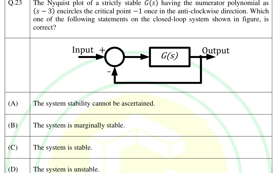
GATE 2025 EE question 23: Unity negative feedback loop. — Figure from the GATE 2025 EE paper. It is part of the question.

(A)
The system stability cannot be ascertained.
(B)
The system is marginally stable.
(C)
The system is stable.
(D)
The system is unstable.

Answer and solution

GATE 2025 EE Q.23: answer and solution

GATE 2025 IN Q.28

GATE 2025 · INQ.28 · 1 mark · MCQ

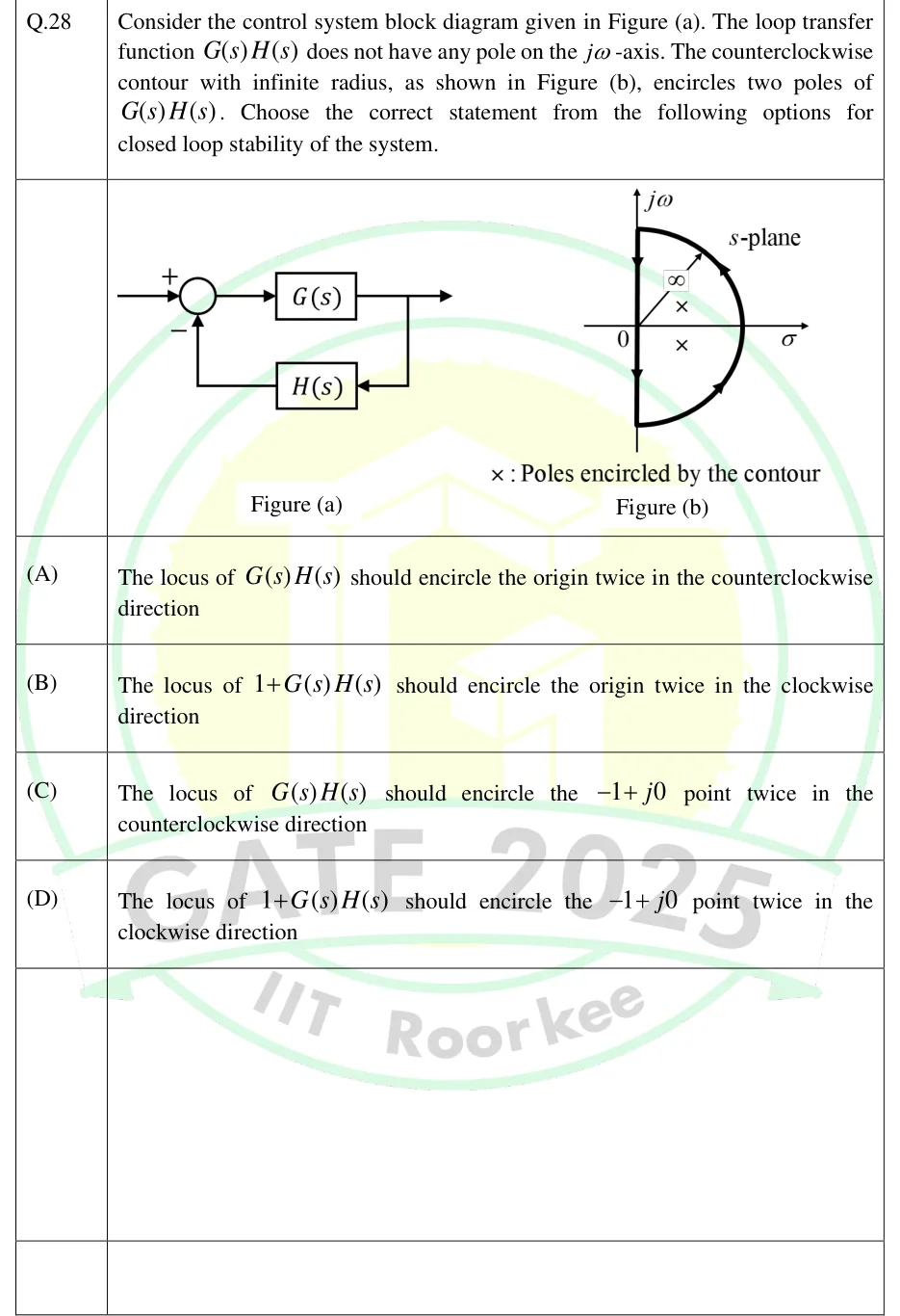
Consider the control system block diagram given in Figure (a). The loop transfer function $G (s) H (s)$ does not have any pole on the $j ω$ -axis. The counterclockwise contour with infinite radius, as shown in Figure (b), encircles two poles of $G (s) H (s)$ . Choose the correct statement from the following options for closed loop stability of the system.

GATE 2025 IN question 28: Figure (a): negative-feedback loop. — Figure from the GATE 2025 IN paper. It is part of the question.

(A)
The locus of $G (s) H (s)$ should encircle the origin twice in the counterclockwise direction
(B)
The locus of $1 + G (s) H (s)$ should encircle the origin twice in the clockwise direction
(C)
The locus of $G (s) H (s)$ should encircle the $- 1 + j 0$ point twice in the counterclockwise direction
(D)
The locus of $1 + G (s) H (s)$ should encircle the $- 1 + j 0$ point twice in the clockwise direction

Answer and solution

GATE 2025 IN Q.28: answer and solution

GATE 2023 EE Q.13

GATE 2023 · EEQ.13 · 1 mark · MCQ

In the Nyquist plot of the open-loop transfer function
$G (s) H (s) = \frac{3 s + 5}{s - 1}$
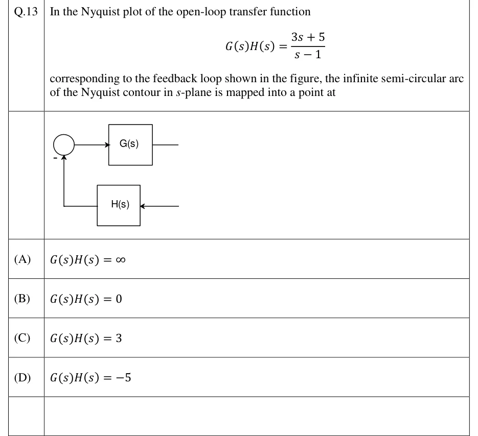
corresponding to the feedback loop shown in the figure, the infinite semi-circular arc of the Nyquist contour in $s$ -plane is mapped into a point at

GATE 2023 EE question 13: Single-loop negative feedback block diagram. — Figure from the GATE 2023 EE paper. It is part of the question.

(A)
$G (s) H (s) = \infty$
(B)
$G (s) H (s) = 0$
(C)
$G (s) H (s) = 3$
(D)
$G (s) H (s) = - 5$

Answer and solution

GATE 2023 EE Q.13: answer and solution

GATE 2023 IN Q.25

GATE 2023 · INQ.25 · 1 mark · NAT

The number of times the Nyquist plot of $G (s) H (s) = \frac{1}{2} \frac{( s - 1 ) ( s - 2 )}{( s + 1 ) ( s + 2 )}$ encircles the origin is ____.

Answer and solution

GATE 2023 IN Q.25: answer and solution

See the question in the paper

Tap to open full size

GATE 2023 IN Q.25: answer and solution

GATE 2022 EC Q.21

GATE 2022 · ECQ.21 · 1 mark · MCQ

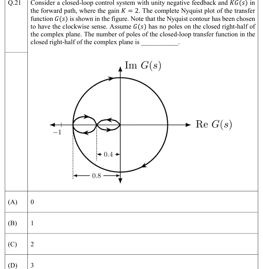
Consider a closed-loop control system with unity negative feedback and $K G (s)$ in the forward path, where the gain $K = 2$ . The complete Nyquist plot of the transfer function $G (s)$ is shown in the figure. Note that the Nyquist contour has been chosen to have the clockwise sense. Assume $G (s)$ has no poles on the closed right-half of the complex plane. The number of poles of the closed-loop transfer function in the closed right-half of the complex plane is ________.

GATE 2022 EC question 21: Nyquist plot of G(s). — Figure from the GATE 2022 EC paper. It is part of the question.

(A)
0
(B)
1
(C)
2
(D)
3

Answer and solution

GATE 2022 EC Q.21: answer and solution

GATE 2022 EE Q.38

GATE 2022 · EEQ.38 · 2 marks · MCQ

The open loop transfer function of a unity gain negative feedback system is given as

G (s) = \frac{1}{s ( s + 1 )} .

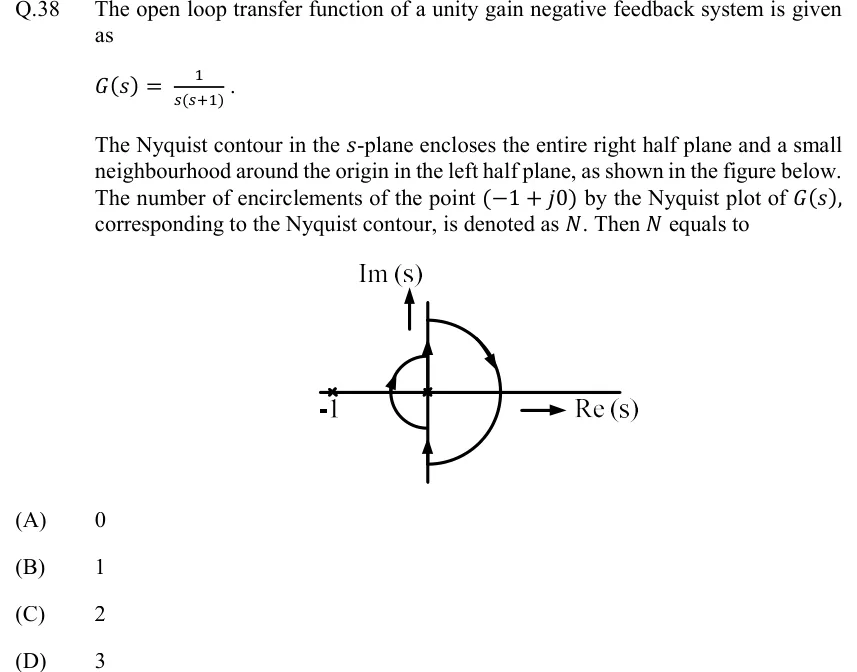
The Nyquist contour in the $s$ -plane encloses the entire right half plane and a small neighbourhood around the origin in the left half plane, as shown in the figure below. The number of encirclements of the point $(- 1 + j 0)$ by the Nyquist plot of $G (s)$ , corresponding to the Nyquist contour, is denoted as $N$ . Then $N$ equals to

GATE 2022 EE question 38: The s-plane has a horizontal axis labelled Re(s) with an arrow pointing right, and a vertical axis labelled Im(s) with an… — Figure from the GATE 2022 EE paper. It is part of the question.

(A)
0
(B)
1
(C)
2
(D)
3

Answer and solution

GATE 2022 EE Q.38: answer and solution

GATE 2020 EC Q.11

GATE 2020 · ECQ.11 · 1 mark · MCQ

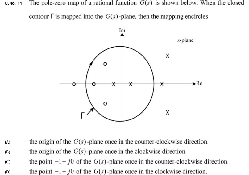
The pole-zero map of a rational function $G (s)$ is shown below. When the closed contour $Γ$ is mapped into the $G (s)$ -plane, then the mapping encircles

GATE 2020 EC question 11: An s-plane with a horizontal axis labelled Re and a vertical axis labelled Im. — Figure from the GATE 2020 EC paper. It is part of the question.

(A)
the origin of the $G (s)$ -plane once in the counter-clockwise direction.
(B)
the origin of the $G (s)$ -plane once in the clockwise direction.
(C)
the point $- 1 + j 0$ of the $G (s)$ -plane once in the counter-clockwise direction.
(D)
the point $- 1 + j 0$ of the $G (s)$ -plane once in the clockwise direction.

Answer and solution

GATE 2020 EC Q.11: answer and solution

GATE 2020 EE Q.24

GATE 2020 · EEQ.24 · 1 mark · NAT

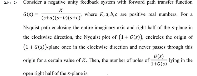
Consider a negative unity feedback system with forward path transfer function $G (s) = \frac{K}{( s + a ) ( s - b ) ( s + c )}$ , where $K, a, b, c$ are positive real numbers. For a Nyquist path enclosing the entire imaginary axis and right half of the $s$ -plane in the clockwise direction, the Nyquist plot of $(1 + G (s))$ , encircles the origin of $(1 + G (s))$ -plane once in the clockwise direction and never passes through this origin for a certain value of $K$ . Then, the number of poles of $\frac{G ( s )}{1 + G ( s )}$ lying in the open right half of the $s$ -plane is ________.

Answer and solution

GATE 2020 EE Q.24: answer and solution

See the question in the paper

Tap to open full size

GATE 2020 EE Q.24: answer and solution

GATE 2020 IN Q.29

GATE 2020 · INQ.29 · 2 marks · MCQ

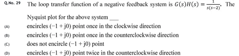
The loop transfer function of a negative feedback system is $G (s) H (s) = \frac{1}{s ( s - 2 )}$ . The Nyquist plot for the above system ____

(A)
encircles $(- 1 + j 0)$ point once in the clockwise direction
(B)
encircles $(- 1 + j 0)$ point once in the counterclockwise direction
(C)
does not encircle $(- 1 + j 0)$ point
(D)
encircles $(- 1 + j 0)$ point twice in the counterclockwise direction

Answer and solution

GATE 2020 IN Q.29: answer and solution

See the question in the paper

Tap to open full size

GATE 2020 IN Q.29: answer and solution

GATE 2018 EC Q.5

GATE 2018 · ECQ.5 · 1 mark · MCQ

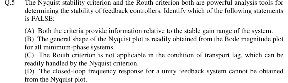
The Nyquist stability criterion and the Routh criterion both are powerful analysis tools for determining the stability of feedback controllers. Identify which of the following statements is FALSE:

(A)
Both the criteria provide information relative to the stable gain range of the system.
(B)
The general shape of the Nyquist plot is readily obtained from the Bode magnitude plot for all minimum-phase systems.
(C)
The Routh criterion is not applicable in the condition of transport lag, which can be readily handled by the Nyquist criterion.
(D)
The closed-loop frequency response for a unity feedback system cannot be obtained from the Nyquist plot.

Answer and solution

GATE 2018 EC Q.5: answer and solution

See the question in the paper

Tap to open full size

GATE 2018 EC Q.5: answer and solution

GATE 2018 IN Q.36

GATE 2018 · INQ.36 · 2 marks · NAT

Consider the standard negative feedback configuration with $G (s) = \frac{s ^{2} + 0.2 s + 100}{s ^{2} - 0.2 s + 100}$ and $H (s) = \frac{1}{2}$ . The number of clockwise encirclements of $(- 1, 0)$ in the Nyquist plot of the Loop transfer-function $G (s) H (s)$ is ______

Answer and solution

GATE 2018 IN Q.36: answer and solution

See the question in the paper

Tap to open full size

GATE 2018 IN Q.36: answer and solution

PRACTICE

5 questions to test yourself

PRACTICE 12 marks · MCQ

A unity-negative-feedback system has $G (s) = \frac{K ( s + 2 )}{( s - 1 ) ( s + 4 )}$ with $K > 0$ . Using the Nyquist criterion, the closed loop is stable for

(A)
$0 < K < 2$ only
(B)
$K > 2$ only
(C)
$K > 4$ only
(D)
no positive value of $K$

Answer and solution

Answer: (B)

$P = 1$ (the pole at $s = + 1$ ). There are no $j ω$ -axis poles, so no indentation is needed. Stability needs $N = - 1$ .
$G (j 0) = \frac{2 K}{- 4} = - \frac{K}{2}$ . The plot meets the negative real axis at $ω = 0$ , where the $ω < 0$ and $ω > 0$ branches join. $G$ is strictly proper, so the large semicircle maps to the origin.
For $ω > 0$ : $∠ G = - 18 0^{\circ} + tan^{- 1} \frac{ω}{2} + tan^{- 1} ω - tan^{- 1} \frac{ω}{4}$ . This stays strictly between $- 18 0^{\circ}$ and $- 8 4^{\circ}$ , so there is no other real-axis crossing.
Just above $ω = 0$ the phase is slightly greater than $- 18 0^{\circ}$ , so the $ω > 0$ branch leaves $- K /2$ into the lower half-plane, and the mirror branch arrives from the upper half-plane. So the plot crosses the negative real axis once, going downward, at $- K /2$ . That crossing is counterclockwise about $- 1$ when $- K /2 < - 1$ .
$K > 2$ : $N = - 1$ , $Z = 0$ , stable. $0 < K < 2$ : $N = 0$ , $Z = 1$ , unstable.
Check: $s^{2} + (3 + K) s + (2 K - 4) = 0$ needs $2 K - 4 > 0$ , i.e. $K > 2$ .

PRACTICE 22 marks · MSQ

A negative-feedback loop has open-loop transfer function $K G_{1} (s) H_{1} (s)$ with $K > 0$ . $G_{1} (s) H_{1} (s)$ is strictly proper and has no poles in the closed right half-plane (none on the $j ω$ -axis either). As $ω$ increases from $0$ to $\infty$ , the plot of $G_{1} (j ω) H_{1} (j ω)$ starts on the positive real axis and crosses the negative real axis exactly three times: at $- 4$ , then $- 2$ , then $- 0.5$ . At $- 4$ and at $- 0.5$ it passes from the third quadrant into the second; at $- 2$ it passes from the second quadrant into the third. For $ω > 0$ it meets the real axis nowhere else. For which of the following values of $K$ is the closed loop stable?

(A)
$K = 0.2$
(B)
$K = 0.4$
(C)
$K = 1$
(D)
$K = 3$

Answer and solution

Answer: (A), (C)

$P = 0$ , so stability needs $N = 0$ . The crossings of $K G_{1} H_{1}$ are at $- 4 K$ , $- 2 K$ and $- 0.5 K$ . The large semicircle maps to the origin, and there is no indentation.
Draw the ray from $- 1$ along the negative real axis. A crossing to the left of $- 1$ from the third into the second quadrant (lower to upper half-plane) is clockwise, and its mirror image adds the same: $+ 2$ . A crossing from the second into the third quadrant is counterclockwise: $- 2$ .
$K = 0.2$ : crossings at $- 0.8$ , $- 0.4$ , $- 0.1$ , none of them left of $- 1$ . $N = 0$ , $Z = 0$ : stable.
$K = 0.4$ : $- 1.6$ is left of $- 1$ ( $+ 2$ ); $- 0.8$ and $- 0.2$ are not. $N = 2$ , $Z = 2$ : unstable.
$K = 1$ : $- 4$ ( $+ 2$ ) and $- 2$ ( $- 2$ ) are left of $- 1$ ; $- 0.5$ is not. $N = 0$ : stable.
$K = 3$ : $- 12$ ( $+ 2$ ), $- 6$ ( $- 2$ ) and $- 1.5$ ( $+ 2$ ). $N = 2$ : unstable. Overall the loop is stable for $0 < K < 0.25$ and $0.5 < K < 2$ , so it is conditionally stable.

PRACTICE 31 mark · MCQ

The open-loop transfer function $G (s) H (s)$ of a negative-feedback system has two poles in the open right half of the $s$ -plane and no poles on the $j ω$ -axis. Its Nyquist plot, drawn for the Nyquist contour traversed clockwise around the right half-plane, does not pass through $- 1 + j 0$ and encircles it once, net, in the counterclockwise direction. The number of closed-loop poles in the right half-plane is

(A)
0
(B)
1
(C)
2
(D)
3

Answer and solution

Answer: (B)

Clockwise-positive convention: one counterclockwise encirclement gives $N = - 1$ , and $P = 2$ .
$Z = N + P = - 1 + 2 = 1$ .
A stable closed loop would need two counterclockwise encirclements ( $N = - 2$ ).

PRACTICE 41 mark · NAT

A negative-feedback system has open-loop transfer function $G (s) H (s) = \frac{8}{s ( s + 1 ) ( s + 4 )}$ . The gain margin read from its Nyquist plot, in dB, is ______ (round off to two decimal places).

Answer and solution

Answer: $7.96$ (accepted range $\pm 0.02$ )

$G H (j ω) = \frac{8}{- 5 ω ^{2} + j ω ( 4 - ω ^{2} )}$ .
Phase crossover: $Im = 0$ gives $ω_{p c}^{2} = 4$ , so $ω_{p c} = 2$ rad/s.
$G H (j 2) = \frac{8}{- 20} = - 0.4$ , so GM $= \frac{1}{0.4} = 2.5$ . The shortcut gives the same: $- \frac{K}{ab ( a + b )} = - \frac{8}{4 \times 5}$ .
GM $_{dB} = 20 lo g_{10} 2.5 \approx 7.96$ dB.

PRACTICE 52 marks · NAT

A unity-negative-feedback loop has $G (s) = \frac{2 e ^{- s T}}{s ( s + 1 )}$ , where $T \geq 0$ is a pure time delay in seconds. The closed loop is stable for $0 \leq T < T_{m a x}$ . The value of $T_{m a x}$ in seconds is ______ (round off to two decimal places).

Answer and solution

Answer: $0.54$ (accepted range $\pm 0.01$ )

The delay does not change $∣ G (j ω) ∣$ , so $ω_{g c}$ is the same as for $\frac{2}{s ( s + 1 )}$ : $\frac{2}{ω ω ^{2} + 1} = 1$ gives $ω^{4} + ω^{2} - 4 = 0$ .
$ω^{2} = \frac{- 1 + 17}{2} \approx 1.5616$ , so $ω_{g c} \approx 1.2496$ rad/s. The magnitude falls monotonically, so this is the only unit-circle crossing.
Without the delay, the closed loop $s^{2} + s + 2$ is stable, and the phase margin is $18 0^{\circ} - 9 0^{\circ} - tan^{- 1} (1.2496) \approx 38.6 7^{\circ} \approx 0.6749$ rad.
The delay adds a lag of $ω T$ . The plot first reaches $- 1$ when $ω_{g c} T$ equals the PM: $T_{m a x} = \frac{0.6749}{1.2496} \approx 0.54$ s.

OFFICIAL GATE 2027 SYLLABUS WORDING

Copied from the GATE 2027 syllabus; see all 2027 syllabi.

GATE EC

Nyquist stability criteria

GATE EE

Stability analysis using … Nyquist criteria

GATE IN

Nyquist criteria

Preparing in Kolkata? IAE Academy's course for GATE ECE, GATE EE or GATE IN.